import numpy as np
import pandas as pd
from collections import OrderedDict
import matplotlib
import matplotlib.pyplot as plt
from matplotlib import gridspec
from matplotlib.colors import ListedColormap, LinearSegmentedColormap, BoundaryNorm
import scipy
from scipy import signal, ndimage
from scipy.interpolate import interp1d
import IPython.display as ipd
from IPython.display import Image, Audio
import librosa
path_img = '../img/9.musically_informed_audio_decomposition/'
path_data = '../data_FMP/'
from utils.plot_tools import *
from utils.feature_tools import f_pitch9.2. 멜로디 추출
Melody Extraction
오디오 분해
멜로디
스펙트로그램
멜로디 추출에 대해 알아보고 그 예를 살펴본다. 또한 순간 주파수 추정, 돌출(salience) 표현, 기본 주파수 추적 등을 설명한다.
이 글은 FMP(Fundamentals of Music Processing) Notebooks을 참고로 합니다.
순간 주파수(Instantaneous Frequency) 추정
다음에서는 순간(instantaneous) 주파수 추정이라는 기술을 소개한다.
기존의 일부 표기법을 수정하여 이산 STFT의 일부 속성을 보자.
\(x\)는 \(F_\mathrm{s}\) 헤르츠의 비율로 샘플링된 주어진 음악 신호를 나타낸다. 또한, \(\mathcal{X}\)를 길이 \(N\in\mathbb{N}\) 및 홉 크기 \(H\in\mathbb{N}\)의 적절한 윈도우 함수를 사용하는 STFT라고 하자.
푸리에 계수 \(\mathcal{X}(n,k)\)의 경우, 프레임 인덱스 \(n\in\mathbb{Z}\)는 물리적 시간 \(T_\mathrm{coef}(n) := \frac{n\cdot H}{F_\mathrm{s}}\) (초 단위)와 관련되어 있다. 주파수 지수 \(k\in[0:N/2]\)는 주파수 $F_(k) := $(헤르츠로 표시)에 해당한다.
특히 이산 STFT는 \(F_\mathrm{s}/N\)Hz의 해상도(resolution)으로 주파수 축의 선형 샘플링을 할 수 있다. 그러나 이 해상도는 특정 시간-주파수 패턴(예: 비브라토 또는 글리산도로 인해 지속적으로 변화하는 패턴)을 정확하게 캡처하는 데 충분하지 않을 수 있다. 또한, 주파수의 로그 인식으로 인해, 주파수 축의 선형 샘플링은 스펙트럼의 저주파(low-frequency) 부분에서 특히 문제가 된다. 단순히 윈도우 길이 \(N\)을 증가시켜 주파수 해상도를 높이는 것은 실행 가능한 솔루션이 아니다. 이 프로세스는 시간적(temporal) 해상도를 감소시키기 때문이다.
다음에서는 복소수 STFT로 인코딩된 위상 정보를 이용하여 향상된 주파수 추정을 얻는 기법에 대해 논의한다.
순간 주파수 (IF)
우선 주파수 표현 및 측정의 주요 아이디어를 상기해보자. 다음 형식의 복소수 지수 함수를 고려한다. \[\mathbf{exp}_{\omega,\varphi}:\mathbb{R}\to\mathbb{C}, \quad \mathbf{exp}_\omega(t):= \mathrm{exp}\big (2\pi i(\omega t - \varphi)\big)\]
- 주파수 매개변수 \(\omega\in\mathbb{R}\)(\(\mathrm{Hz}\)로 측정) 및 위상 매개변수 \(\varphi\)(\(360^\circ\)의 각도에 해당하는 \(1\)로 정규화된 라디안으로 측정
\(\varphi=0\)인 경우, \[\mathbf{exp}_{\omega} := \mathbf{exp}_{\omega,0}\]
시간 매개변수 \(t\)를 균일하게 증가시키면, 지수 함수는 단위 원(unit circle) 주위의 원 운동(circular motion)을 설명한다. 실제 및 가상 축에 투영하면 두 개의 정현파 운동(sinusoidal motions)(코사인 및 사인 함수로 설명됨)이 생성된다.
원형 운동을 균일하게 회전하는 바퀴로 생각하면 주파수 매개변수 \(\omega\)는 단위 시간당 회전 수(이 경우 1초 지속 시간)에 해당한다. 즉, 주파수는 회전율로 해석할 수 있다.
이 해석을 기반으로 임의의 시간 간격 \([t_1,t_2]\) 및 \(t_1<t_2\) 동안 회전하는 바퀴와 주파수 값을 연결할 수 있다. 이를 위해 시간 \(t_1\)에서의 각도 위치 \(\varphi_1\)와 시간 \(t_2\)에서의 각도 위치 \(\varphi_2\)를 측정한다. 이는 다음 그림에 설명되어 있다.
Image(path_img+"FMP_C8_F12.png", width=300)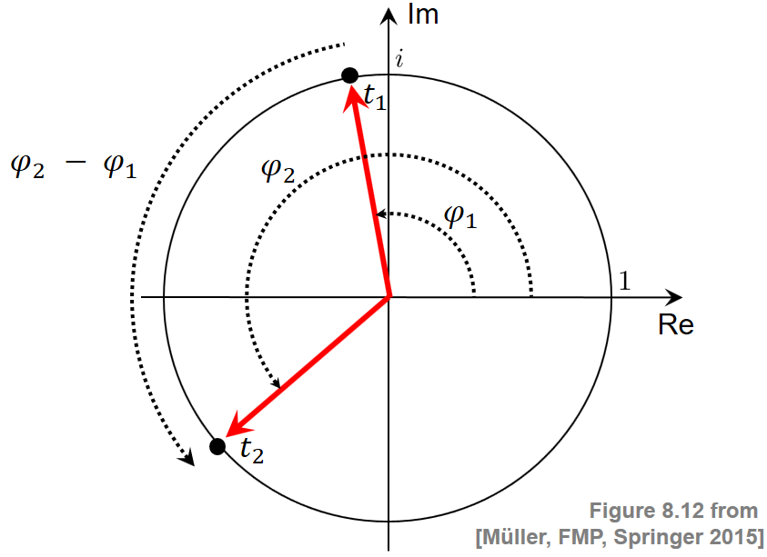
주파수는 시간 간격의 길이 \(t_2-t_1\)로 나눈 각도 위치의 변화 \(\varphi_2-\varphi_1\)로 정의된다.
극한의 경우, 시간 간격이 임의로 작아지면 다음과 같이 주어진 순간 주파수 \(\omega_{t_1}\)를 얻는다. \[\omega_{t_1}:=\lim_{t_2\to t_1}\frac{\varphi_2-\varphi_1}{t_2-t_1}\]
위상 예측 오류
주파수 값 \(\omega\in\mathbb{R}\)과 두 개의 시간 인스턴스(\(t_1\in\mathbb{R}\), \(t_2\in\mathbb{R}\))를 고정하는 시간-연속적 관점을 가정해 보자.
나중에 STFT 매개변수와 관련된 특정 값을 선택할 것이다. 신호 \(x\)를 윈도우 버전의 분석 함수 \(\mathbf{exp}_\omega\)(하나는 \(t_1\)에, 다른 하나는 \(t_2\)에 위치)와 연관시키면, 두 개의 복소 푸리에 계수를 얻는다.
\(\varphi_1\)와 \(\varphi_2\)를 각각 이 두 계수의 위상이라 하자.
신호 \(x\)가 주파수 \(\omega\)의 강한 주파수 성분을 포함하는 경우, \(\varphi_1\) 및 \(\varphi_2\)의 두 위상은 다음과 같은 방식으로 일치해야 한다. : 시간 위치 \(t_1\)에서 각도 위치 \(\varphi_1\)를 가정하는 주파수 \(\omega\)의 회전(rotation)이 시간 \(t_2\)에서 위상 \(\varphi^\mathrm{Pred}:=\varphi_1 + \omega\cdot \Delta t\)를 가져야 한다.(\(\Delta t:=t_2-t_1\))
따라서 신호 \(x\)가 함수 \(\mathbf{exp}_\omega\)와 유사하게 동작하는 경우 \(\varphi_2\approx\varphi^\mathrm{Pred}\)이어야 한다. \(x\) 신호가 \(\mathbf{exp}_\omega\)보다 약간 느리게 진동(oscillate)하는 경우 \(x\) 신호에 대한 인스턴스 \(t_1\)에서 인스턴스 \(t_2\)까지의 위상 증분은 프로토타입 진동 \(\mathbf{exp}_\omega\)에 대한 것보다 작다. 결과적으로 \(t_2\)에서 측정된 위상 \(\varphi_2\)는 예측 위상 \(\varphi^\mathrm{Pred}\)보다 작다. \(x\)가 \(\mathbf{exp}_\omega\)보다 약간 빠르게 진동하는 세 번째 경우에서 \(\varphi_2\) 위상은 예측 위상 \(\varphi^\mathrm{Pred}\)보다 크다. 세 가지 경우를 다음 그림으로 설명한다.
Image(path_img+"FMP_C8_F13.png", width=300)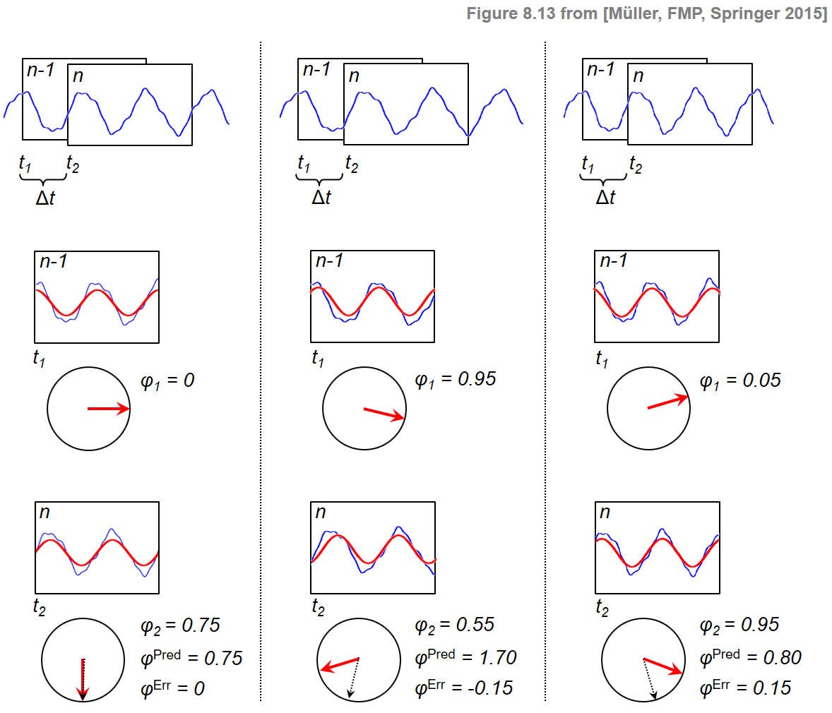
\(\varphi_2\)와 \(\varphi^\mathrm{Pred}\)의 차이를 측정하기 위해 다음과 같이 정의된 예측 오류를 도입한다. \[\varphi^\mathrm{Err}:=\Psi(\varphi_2-\varphi^\mathrm{Pred})\]
이 정의에서 \(\Psi:\mathbb{R}\to\left[-0.5,0.5\right]\)는 principal argument function이며, 적절한 정수 값을 더하거나 빼서 위상차를 \([-0.5,0.5]\) 범위로 매핑한다. 이는 위상 차이를 계산할 때 불연속성을 방지한다.
예측 오류는 신호 \(x\)에 대한 정제된 주파수 추정 \(\mathrm{IF}(\omega)\)를 얻기 위해 주파수 값 \(\omega\)를 수정하는 데 사용할 수 있다. \[\mathrm{IF}(\omega) := \omega + \frac{\varphi^\mathrm{Err}}{\Delta t}\]
이 값은 순간 주파수(instantaneous frequency)(IF)라고도 하며 초기 주파수 \(\omega\)의 조정으로 생각할 수 있다. 엄밀히 말하면, 순간 빈도는 단일 시간 인스턴스를 참조하는 것이 아니라 전체 시간 간격 \([t_1,t_2]\)를 참조한다. 그러나 실제로 이 간격은 일반적으로 매우 작게 선택된다(대략 몇 밀리초(milliseconds)).
STFT 주파수 해상도 개선
이제 이산 STFT의 주파수 해상도를 개선하기 위해 순간 주파수 개념을 적용한다. 극좌표 표현을 사용하여 푸리에 계수 \(\mathcal{X}(n,k)\in\mathbb{C}\)를 다음과 같이 쓸 수 있다. \[\mathcal{X}(n,k)= |\mathcal{X}(n,k)|\mathrm{exp}(2\pi i\varphi(n,k))\] for \(\varphi(n,k)\in[0,1)\)
프로토타입 진동의 경우, 주파수 매개변수 \(k\in[0:N/2]\)에 의해 결정되는 주파수를 사용한다. \[\omega = F_\mathrm{coef}(k) = \frac{k\cdot F_\mathrm{s}}{N}.\]
또한 두 시간 인스턴스는 이전 프레임과 현재 프레임의 위치에 따라 결정된다. \[t_1=T_\mathrm{coef}(n-1)=\frac{(n-1)\cdot H}{F_\mathrm{s}},\] \[\quad t_2=T_\mathrm{coef}(n)=\frac{n\cdot H}{F_\mathrm{s}}\]
마지막으로 이러한 시간 인스턴스에서 측정된 위상은 STFT에서 얻은 것이다. \[\varphi_1=\varphi(n-1,k)\] \[\varphi_2=\varphi(n,k)\]
이로부터 위의 방정식들을 사용하고 약간의 재정렬을 수행하여 순간 주파수를 얻는다. \[F_\mathrm{coef}^\mathrm{IF}(k,n):=\mathrm{IF}(\omega) = \left( k + \kappa(k,n) \right)\cdot\frac{F_\mathrm{s}}{N}\] bin offset \(\kappa(k,n) = \frac{N}{H}\cdot\Psi\left(\varphi(n,k)-\varphi(n-1,k) - \frac{k\cdot H}{N}\right)\)
구현
- 다음 코드 셀에서는 주어진 STFT의 모든 시간-주파수 빈에 대한 순간 주파수(IF)를 추정하는 구현을 제공한다.
- 입력은 샘플링 속도
Fs, 윈도우 길이N, 홉 크기H, 그리고 차원K(주파수 빈 수) 및L(프레임 수)의 복소수 값 STFT 행렬X로 구성된다. - 출력은 각 시간-주파수 빈에 대한 IF의 추정치를 포함하는 실수 값 행렬
F_coef_IF이다.F_coef_IF도 (K\(\times\)L)-행렬이 되도록 패딩을 적용한다. - 구현에서 IF는 행렬 연산을 사용하여 모든 시간-주파수 빈에 대해 동시에 계산된다.
- 입력은 샘플링 속도
def principal_argument(v):
"""Principal argument function
Args:
v (float or np.ndarray): Value (or vector of values)
Returns:
w (float or np.ndarray): Principle value of v
"""
w = np.mod(v + 0.5, 1) - 0.5
return w
def compute_if(X, Fs, N, H):
"""Instantenous frequency (IF) estamation
Args:
X (np.ndarray): STFT
Fs (scalar): Sampling rate
N (int): Window size in samples
H (int): Hop size in samples
Returns:
F_coef_IF (np.ndarray): Matrix of IF values
"""
phi_1 = np.angle(X[:, 0:-1]) / (2 * np.pi)
phi_2 = np.angle(X[:, 1:]) / (2 * np.pi)
K = X.shape[0]
index_k = np.arange(0, K).reshape(-1, 1)
# Bin offset (FMP, Eq. (8.45))
kappa = (N / H) * principal_argument(phi_2 - phi_1 - index_k * H / N)
# Instantaneous frequencies (FMP, Eq. (8.44))
F_coef_IF = (index_k + kappa) * Fs / N
# Extend F_coef_IF by copying first column to match dimensions of X
F_coef_IF = np.hstack((np.copy(F_coef_IF[:, 0]).reshape(-1, 1), F_coef_IF))
return F_coef_IFIF 시각화
- 이제 IF 추정 절차에 대한 더 깊은 통찰력을 제공하는 시각화를 소개한다. 예를 들어, 피아노로 연주되는 \(\mathrm{C4}\)의 단일 음 또는 녹음을 고려하자. 이 음은 중심 주파수가 \(261.6~\mathrm{Hz}\), MIDI 피치 \(p=60\)에 해당한다. 다음 그림은 오디오 신호의 파형과 스펙트로그램 표현을 보여준다.
fn_wav = 'FMP_C6_F04_NoteC4_Piano.wav'
x, Fs = librosa.load(path_data+fn_wav)
ipd.display(Audio(data=x,rate=Fs))
N = 2048
H = 64
X = librosa.stft(x, n_fft=N, hop_length=H, win_length=N, window='hann')
Y = np.log(1+ 10*np.abs(X))
K = X.shape[0]
L = X.shape[1]
ylim = [0,1500]
fig, ax = plt.subplots(2, 2, gridspec_kw={'width_ratios': [1, 0.05],
'height_ratios': [1, 2]}, figsize=(5, 4))
plot_signal(x, Fs, ax=ax[0,0])
ax[0,1].set_axis_off()
plot_matrix(Y, Fs=Fs/H, Fs_F=N/Fs, ax=[ax[1,0],ax[1,1]], colorbar=True)
ax[1,0].set_ylim(ylim)
plt.tight_layout()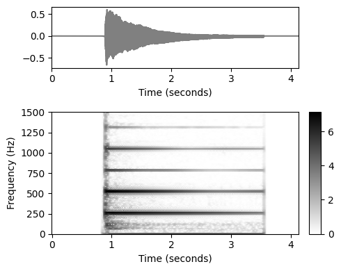
IF 추정의 출력은 주파수 값 \(F_\mathrm{coef}^\mathrm{IF}(k,n)\in\mathbb{R}\)(Hertz로 제공됨)이다(\(k\in[0:K-1]\), \(n\in[0:L-1]\)). 이 값은 STFT의 \(k\)번째 푸리에 계수와 관련된 (프레임 독립적인) 주파수 값 \(F_\mathrm{th}\)의 개선이다.
다음 그림에서 \(F_\mathrm{coef}\) 및 \(F_\mathrm{coef}^\mathrm{IF}\)에 의해 주어진 \((K\times N)\)-행렬을 색상 코드 형태로 표시한다. 또한 Hertz로 지정된 bin offset인 차이를 시각화한다. \[F_\mathrm{coef}^\mathrm{IF}-F_\mathrm{coef} = \kappa \cdot\frac{N}{F_\mathrm{s}}\]
스펙트로그램을 시각화(크기(magnitude)가 색상으로 구분됨)하는 것과 반대로 이번에는 주파수 값을 시각화(헤르츠로 표시됨)한다.
def plot_IF(F_coef_X, F_coef_IF, ylim, figsize=(10,3)):
plt.figure(figsize=figsize)
ax = plt.subplot(1,3,1)
plot_matrix(F_coef_X, Fs=Fs/H, Fs_F=N/Fs, cmap='PuOr', clim=ylim, ax=[ax],
title=r'$F_\mathrm{coef}$')
plt.ylim(ylim)
ax = plt.subplot(1,3,2)
plot_matrix(F_coef_IF, Fs=Fs/H, Fs_F=N/Fs, cmap='PuOr', clim=ylim, ax=[ax],
title=r'$F_\mathrm{coef}^\mathrm{IF}$')
plt.ylim(ylim)
ax = plt.subplot(1,3,3)
plot_matrix(F_coef_IF-F_coef_X, Fs=Fs/H, Fs_F=N/Fs, cmap='seismic', ax=[ax],
title=r'$F_\mathrm{coef}^\mathrm{IF}-F_\mathrm{coef}$')
plt.ylim(ylim)
plt.tight_layout()
F_coef_IF = compute_if(X, Fs, N, H)
F_coef = np.arange(K) * Fs / N
F_coef_X = np.ones((K,L)) * F_coef.reshape(-1,1)
plot_IF(F_coef_X, F_coef_IF, ylim) 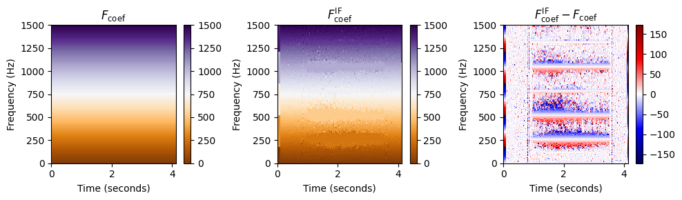
이 시각화에서 행렬 \(F_\mathrm{coef}\)와 \(F_\mathrm{coef}^\mathrm{IF}\)는 상당히 유사해 보인다. 그러나 차이를 볼 때 음표 \(\mathrm{C4}\) (\(261.6~\mathrm{Hz}\))의 기본 주파수와 그 고조파의 영역에서 주파수 값의 조정을 명확하게 볼 수 있다.
고조파 바로 아래의 주파수 값은 위로 조정되고(빨간색) 고조파 바로 위의 주파수 값은 아래로 보정된다(파란색).
다음 그림에서는 주파수 값에 대한 색상 코딩을 조정하면서 기본 주파수 \(261.6~\mathrm{Hz}\) 부근을 확대한다. 이 시각화는 IF 추정 절차가 \(261.6~\mathrm{Hz}\) 부근의 모든 주파수 계수를 정확히 해당 주파수에 할당함을 보여준다.
# Compute a neighborhood around center frequency of C4 (p=60)
pitch = 60
freq_fund = 2 ** ((pitch - 69) / 12) * 440
freq_0 = freq_fund-150
freq_1 = freq_fund+150
ylim = [freq_0, freq_1]
plot_IF(F_coef_X, F_coef_IF, ylim) 
홉 크기에 따라서
추정된 순간 주파수의 품질은 다음의 두 연속된 프레임 사이의 길이에 따라 달라진다. \[\Delta t=t_2-t_1 = T_\mathrm{coef}(n) - T_\mathrm{coef}(n-1) = H/F_\mathrm{s}\]
따라서 이산 STFT에 적용할 때 작은 홉 크기 \(H\)를 사용하는 것이 유리하다. 이는 다음 그림에 설명되어 있다. 단, 단점은 작은 홉 크기를 사용하면 이산 STFT를 계산하기 위한 계산 비용이 증가한다는 것이다.
import time
def compute_plot_IF(x, N, H):
# Compute STFT
start = time.time()
X = librosa.stft(x, n_fft=N, hop_length=H, win_length=N, window='hann')
Y = np.log(1+ 10*np.abs(X))
end = time.time()
print('Runtime (STFT): %.8f seconds' % (end - start))
K = X.shape[0]
L = X.shape[1]
# Compute IF
start = time.time()
F_coef_IF = compute_if(X, Fs, N, H)
end = time.time()
print('Runtime (IF): %.8f seconds' % (end - start))
# Plot
F_coef = np.arange(K) * Fs / N
F_coef_X = np.ones((K,L)) * F_coef.reshape(-1,1)
plot_IF(F_coef_X, F_coef_IF, ylim)
plt.show()
N, H = 2048, 64
print('Instanteneous frequency estimation using N=%d and H=%d'%(N,H))
compute_plot_IF(x, N, H)
N, H = 2048, 256
print('Instanteneous frequency estimation using N=%d and H=%d'%(N,H))
compute_plot_IF(x, N, H)
N, H = 2048, 1024
print('Instanteneous frequency estimation using N=%d and H=%d'%(N,H))
compute_plot_IF(x, N, H)Instanteneous frequency estimation using N=2048 and H=64
Runtime (STFT): 0.03986549 seconds
Runtime (IF): 0.15757895 seconds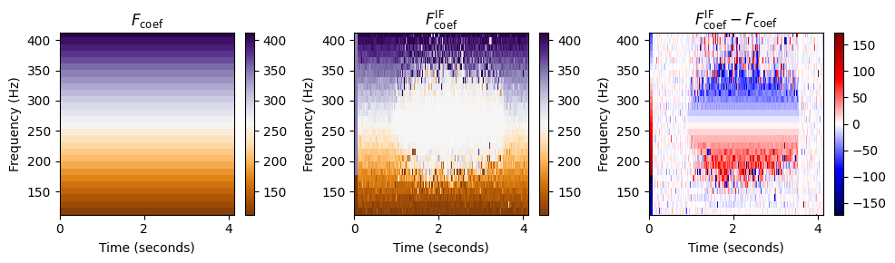
Instanteneous frequency estimation using N=2048 and H=256
Runtime (STFT): 0.00999880 seconds
Runtime (IF): 0.03590417 seconds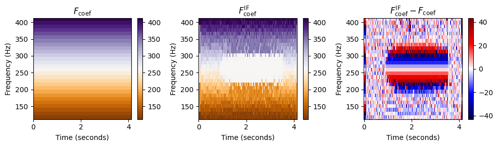
Instanteneous frequency estimation using N=2048 and H=1024
Runtime (STFT): 0.00299215 seconds
Runtime (IF): 0.00797868 seconds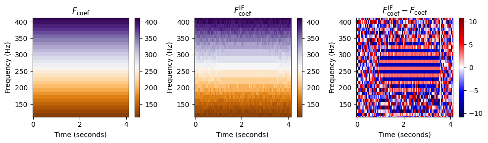
돌출(Salience) 표현
- 향상된 로그-주파수 스펙트로그램인 돌출(salience) 표현을 소개한다.
# 사용할 예시 오디오
ipd.display(Image(path_img+"FMP_C8_F10a.png", width=300))
fn_wav = "FMP_C8_F10_Weber_Freischuetz-06_FreiDi-35-40.wav"
ipd.display(Audio(path_data+fn_wav))
- 다음 그림은 오디오 발췌 부분의 로그 압축된 스펙트로그램과 확대된 시간-주파수 섹션을 보여준다. 사용할 순간 주파수를 고려하여 상대적으로 작은 홉 크기 파라미터 \(H\)를 선택했다.
x, Fs = librosa.load(path_data+fn_wav)
# Computation of STFT
N = 1024
H = 128
X = librosa.stft(x, n_fft=N, hop_length=H, win_length=N, pad_mode='constant')
gamma = 1
Y = np.log(1 + gamma * np.abs(X))
figsize = (10,4)
fig, ax = plt.subplots(1, 2, gridspec_kw={'width_ratios': [2, 1]}, figsize=figsize)
ylim_zoom_pitch = [65, 90]
ylim_zoom = [f_pitch(ylim_zoom_pitch[0]), f_pitch(ylim_zoom_pitch[1])]
xlim_zoom = [0,1]
cmap = compressed_gray_cmap(alpha=5)
plot_matrix(Y, Fs=Fs/H, Fs_F=N/Fs, ax=[ax[0]], title='Spectrogram',
colorbar=True, cmap=cmap);
ax[0].set_ylim([0, 5000])
plot_matrix(Y, Fs=Fs/H, Fs_F=N/Fs, ax=[ax[1]], title='',
colorbar=True, cmap=cmap);
ax[1].set_ylim(ylim_zoom)
ax[1].set_xlim(xlim_zoom)
plt.tight_layout()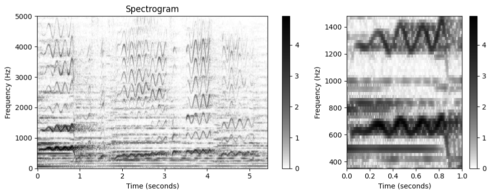
로그-주파수 스펙트로그램 경우
로그-주파수 스펙트로그램을 생각해보자. \(x\)는 \(F_\mathrm{s}\) 레이트로 샘플링되고 윈도우 길이 \(N\in\mathbb{N}\) 및 홉 크기 \(H\in\mathbb{N}\)를 사용한 STFT \(\mathcal{X}\) 오디오 신호를 나타낸다. 주파수 지수 \(k\in[0:N/2]\)는 \(F_\mathrm{coef}(k) := \frac{k\cdot F_\mathrm{s}}{N}\) (헤르츠로 주어짐)에 해당한다.
로그 주파수 스펙트로그램을 얻기 위한 한 가지 전략은 피치 매개변수 \(p\in[0:127]\)에 대한 집합 \(P(p) := \{k:F_\mathrm{MIDI}(p-0.5) \leq F_\mathrm{coef}(k) < F_\mathrm{MIDI}(p+0.5)\}\)에 관한 STFT 계수를 풀링(pool)하거나 비닝(bin)하는 것이다.
중심 주파수는 $ F_(p) = 2^{(p-69)/12} $로 주어진다.
피치를 고정하고 결과 피치 밴드에 있는 모든 주파수를 찾는 대신, 주어진 주파수로 피치 인덱스를 할당하는 \(\mathrm{Bin}:\mathbb{R}\to\mathbb{Z}\) 매핑을 정의할 수도 있다.: \[\mathrm{Bin}(\omega) := \left\lfloor 12\cdot\log_2\left(\frac{\omega}{440}\right)+69.5\right\rfloor.\]
이 함수를 이용하여 비닝(binning)을 다음과 같이 표현할 수 있다. \[P(p) := \{k: \mathrm{Bin}(F_\mathrm{coef}(k))=p\}\]
여기에서 풀링을 통해 로그 주파수 스펙트로그램 \(\mathcal{Y}_\mathrm{LF}:\mathbb{Z}\times [0:127]\)를 얻는다. \[\mathcal{Y}_\mathrm{LF}(n,p) := \sum_{k \in P(p)}{|\mathcal{X}(n,k)|^2}\]
def f_coef(k, Fs, N):
"""STFT center frequency
Args:
k (int): Coefficient number
Fs (scalar): Sampling rate in Hz
N (int): Window length in samples
Returns:
freq (float): STFT center frequency
"""
return k * Fs / N
def frequency_to_bin_index(F, R=10.0, F_ref=55.0):
"""| Binning function with variable frequency resolution
| Note: Indexing starts with 0 (opposed to [FMP, Eq. (8.49)])
Args:
F (float): Frequency in Hz
R (float): Frequency resolution in cents (Default value = 10.0)
F_ref (float): Reference frequency in Hz (Default value = 55.0)
Returns:
bin_index (int): Index for bin (starting with index 0)
"""
bin_index = np.floor((1200 / R) * np.log2(F / F_ref) + 0.5).astype(np.int64)
return bin_index
def p_bin(b, freq, R=10.0, F_ref=55.0):
"""Computes binning mask [FMP, Eq. (8.50)]
Args:
b (int): Bin index
freq (float): Center frequency
R (float): Frequency resolution in cents (Default value = 10.0)
F_ref (float): Reference frequency in Hz (Default value = 55.0)
Returns:
mask (float): Binning mask
"""
mask = frequency_to_bin_index(freq, R, F_ref) == b
mask = mask.reshape(-1, 1)
return mask
def compute_y_lf_bin(Y, Fs, N, R=10.0, F_min=55.0, F_max=1760.0):
"""Log-frequency Spectrogram with variable frequency resolution using binning
Args:
Y (np.ndarray): Magnitude spectrogram
Fs (scalar): Sampling rate in Hz
N (int): Window length in samples
R (float): Frequency resolution in cents (Default value = 10.0)
F_min (float): Lower frequency bound (reference frequency) (Default value = 55.0)
F_max (float): Upper frequency bound (is included) (Default value = 1760.0)
Returns:
Y_LF_bin (np.ndarray): Binned log-frequency spectrogram
F_coef_hertz (np.ndarray): Frequency axis in Hz
F_coef_cents (np.ndarray): Frequency axis in cents
"""
# [FMP, Eq. (8.51)]
B = frequency_to_bin_index(np.array([F_max]), R, F_min)[0] + 1
F_coef_hertz = 2 ** (np.arange(0, B) * R / 1200) * F_min
F_coef_cents = np.arange(0, B*R, R)
Y_LF_bin = np.zeros((B, Y.shape[1]))
K = Y.shape[0]
freq = f_coef(np.arange(0, K), Fs, N)
freq_lim_idx = np.where(np.logical_and(freq >= F_min, freq <= F_max))[0]
freq_lim = freq[freq_lim_idx]
Y_lim = Y[freq_lim_idx, :]
for b in range(B):
coef_mask = p_bin(b, freq_lim, R, F_min)
Y_LF_bin[b, :] = (Y_lim*coef_mask).sum(axis=0)
return Y_LF_bin, F_coef_hertz, F_coef_cents- 다음 코드 셀은 Freischütz예의 로그-주파수 스펙토그램을 나타낸다.
Y_LF, F_coef_hertz, F_coef_cents = compute_y_lf_bin(Y, Fs, N, R=100, F_min=32.703, F_max=11025)
fig, ax = plt.subplots(1, 2, gridspec_kw={'width_ratios': [2, 1]}, figsize=figsize)
plot_matrix(Y_LF, Fs=Fs/H, Fs_F=1, ax=[ax[0]], ylabel='Frequency (pitch)',
title='LF-spectrogram (semitone resolution)',
colorbar=True, cmap=cmap);
ax[0].set_ylim([33, 110])
plot_matrix(Y_LF, Fs=Fs/H, Fs_F=1, ax=[ax[1]], ylabel='Frequency (pitch)',
title='', colorbar=True, cmap=cmap);
ax[1].set_ylim(ylim_zoom_pitch)
ax[1].set_xlim(xlim_zoom)
plt.tight_layout()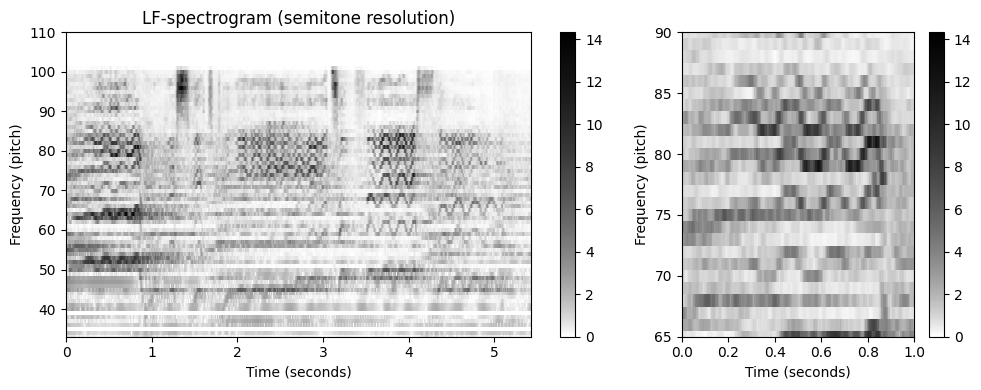
Refined Binning
이제 보다 일반적인 빈 할당(bin assignment)을 고려하여 로그 주파수 스펙트로그램의 정의를 확장한다.
이를 위해 \(\omega_\mathrm{ref}\in\mathbb{R}\)를 빈 인덱스 \(1\)에 할당할 참고 주파수라 하자. 또한, \(R\in\mathbb{R}\)(센트 단위)를 대수적(loagrithmically)으로 간격을 둔 주파수 축의 원하는 해상도(resolution)라고 하자.
그러면 주파수 \(\omega\in\mathbb{R}\)(Hertz로 표시)에 대해 빈(bin) 인덱스 \(\mathrm{Bin}(\omega)\)는 다음과 같이 정의된다. \[\mathrm{Bin}(\omega) := \left\lfloor \frac{1200}{R} \cdot\log_2\left(\frac{\omega}{\omega_\mathrm{ref}}\right)+1.5\right\rfloor\]
예를 들어, \(R=100\)는 빈당 \(100\) 센트(1반음)의 해상도로 주파수 축의 세분화를 산출한다. \(R=10\)을 사용하면 각 빈이 \(10\) 센트(반음의 10분의 1)에 해당하도록 더 미세하게 세분화된다.
빈 매핑 함수를 기반으로 위의 로그 주파수 스펙트로그램의 정의를 확장해보자. 참조 주파수 \(\omega_\mathrm{ref}\) 및 해상도 \(R\)을 고정하고 \(B\in\mathbb{N}\)를 고려할 빈의 수로 둔다. 각 빈 인덱스 \(b\in[1:B]\)에 대해 다음의 집합을 정의한다. \[P(b) := \left\{k: \mathrm{Bin}\left(F_\mathrm{coef}{(k)}\right)=b\right\}\]
또한 스펙트로그램 \(\mathcal{Y} = |\mathcal{X}(n,k)|^2\)(또는 이것의 로그 압축 버전)에서 시작하여, 각 프레임 인덱스 \(n\in\mathbb{Z}\)와 빈 인덱스 \(b\in[1:B]\)에 대해 $ (n,b) := {k P(b)}{(n,k)}$를 설정한다.
이 정제된 비닝 전략은 다음 코드 셀에서 구현된다. 다음 사항에 유의하자.
- 위에서 계산한 로그 압축 스펙트로그램을 입력으로 사용한다.
- \(\omega_\mathrm{min}=55~\mathrm{Hz}\)(피치 \(p=33\)에 해당)와 \(\omega_\mathrm{max}=1760~\mathrm{Hz}\)(피치 \(p=93\)에 해당) 사이의 주파수만 고려된다. 이 범위는 5옥타브(\(6000\) 센트에 해당)를 포함한다.
- 비닝 인덱스 \(b\in[1:B]\)의 경우 파이썬 구현에서 인덱스 0으로 인덱싱을 시작하기 때문에, 주어진 알고리즘 설명과 관련하여 인덱스 이동을 -1로 이끈다.
- 참조 주파수는 \(\omega_\mathrm{ref}= \omega_\mathrm{min}\)로 설정되고 능해도는 \(R=50\) 센트로 설정된다.
- 로그 주파수 스펙트로그램의 시각화에서 주파수 축은 센트 단위로 지정된다(\(0\) 센트는 \(\omega_\mathrm{ref}=55~\mathrm{Hz}\)에 해당됨).
- 특히 낮은 주파수의 경우 STFT에 의해 도입된 선형 주파수 그리드로 인해 빈이 비어 있을 수 있다. 빈(empty) 빈(bin) 문제는 주파수 그리드 해상도를 높이거나 보간 기술을 사용하여 해결할 수 있다.
R = 50
F_min = 55.0
F_max = 1760.0
fig, ax = plt.subplots(1, 2, gridspec_kw={'width_ratios': [2, 1]}, figsize=figsize)
Y_LF_bin, F_coef_hertz, F_coef_cents = compute_y_lf_bin(Y, Fs, N, R, F_min=F_min, F_max=F_max)
plot_matrix(Y_LF_bin, Fs=Fs/H, F_coef=F_coef_cents, ax=[ax[0]], ylabel='Frequency (cents)',
title='LF-spectrogram (R = 50 cents)', colorbar=True, cmap=cmap);
plot_matrix(Y_LF_bin, Fs=Fs/H, F_coef=F_coef_cents, ax=[ax[1]], ylabel='Frequency (cents)',
title='', colorbar=True, cmap=cmap);
ylim_zoom_cents = [3200, 5700]
xlim_zoom = [0,1]
ax[1].set_xlim(xlim_zoom)
ax[1].set_ylim(ylim_zoom_cents)
plt.tight_layout()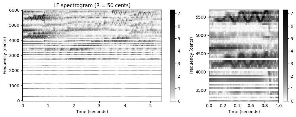
순간 주파수 사용
위에서 소개한 단순 비닝 접근 방식에서는 \(\mathcal{Y}\)의 선형 간격 주파수 정보가 비선형, 로그 방식으로 확장된다. 이것은 특히 \(\mathcal{Y}_\mathrm{LF}\)의 아래쪽 부분에서 볼 수 있는 주파수 방향의 아티팩트(예: 가로 흰색 줄무늬)를 초래한다. 이제 순간 주파수를 사용하여 이 문제를 완화할 수 있는 방법에 대해 논의해본다.
중심 주파수 \(F_\mathrm{coef}(k)\)를 사용하는 대신, 집합 \(P^\mathrm{IF}(b,n) := \left\{k: \mathrm{Bin}\left(F_\mathrm{coef}^\mathrm{IF}(k, n)\right)=b\right\}\) (\(b\in[1:B]\), \(n\in\mathbb{Z}\))을 정의하는 정제된(refined) 주파수 추정치 \(F_\mathrm{coef}^\mathrm{IF}(k,n)\)를 사용한다.
이 새로운 빈 할당에서 다음을 설정하여 정제된 로그 주파수 스펙트로그램 \(\mathcal{Y}_\mathrm{LF}^\mathrm{IF}\)를 도출한다. \[\mathcal{Y}_\mathrm{LF}^\mathrm{IF}(n,b) := \sum_{k \in P^\mathrm{IF}(b,n)}{\mathcal{Y} (n,k)}\] (각 프레임 인덱스 \(n\in\mathbb{Z}\) 및 빈 인덱스 \(b\in[1:B]\)에 대해)
이 수정의 효과는 다음 코드 셀에 설명되어 있다. 순간 주파수를 사용하면 STFT의 선형 주파수 그리드가 초래한 일부 문제가 완화된다. 특히 시간-주파수 패턴은 스펙트럼 계수가 단일 고조파 소스(source)에 명확하게 할당될 수 있을 때 더 선명해진다.
def p_bin_if(b, F_coef_IF, R=10.0, F_ref=55.0):
"""Computes binning mask for instantaneous frequency binning [FMP, Eq. (8.52)]
Args:
b (int): Bin index
F_coef_IF (float): Instantaneous frequencies
R (float): Frequency resolution in cents (Default value = 10.0)
F_ref (float): Reference frequency in Hz (Default value = 55.0)
Returns:
mask (np.ndarray): Binning mask
"""
mask = frequency_to_bin_index(F_coef_IF, R, F_ref) == b
return mask
def compute_y_lf_if_bin(X, Fs, N, H, R=10, F_min=55.0, F_max=1760.0, gamma=0.0):
"""Binned Log-frequency Spectrogram with variable frequency resolution based on instantaneous frequency
Args:
X (np.ndarray): Complex spectrogram
Fs (scalar): Sampling rate in Hz
N (int): Window length in samples
H (int): Hopsize in samples
R (float): Frequency resolution in cents (Default value = 10)
F_min (float): Lower frequency bound (reference frequency) (Default value = 55.0)
F_max (float): Upper frequency bound (Default value = 1760.0)
gamma (float): Logarithmic compression factor (Default value = 0.0)
Returns:
Y_LF_IF_bin (np.ndarray): Binned log-frequency spectrogram using instantaneous frequency
F_coef_hertz (np.ndarray): Frequency axis in Hz
F_coef_cents (np.ndarray): Frequency axis in cents
"""
# Compute instantaneous frequencies
F_coef_IF = compute_if(X, Fs, N, H)
freq_lim_mask = np.logical_and(F_coef_IF >= F_min, F_coef_IF < F_max)
F_coef_IF = F_coef_IF * freq_lim_mask
# Initialize ouput array and compute frequency axis
B = frequency_to_bin_index(np.array([F_max]), R, F_min)[0] + 1
F_coef_hertz = 2 ** (np.arange(0, B) * R / 1200) * F_min
F_coef_cents = np.arange(0, B*R, R)
Y_LF_IF_bin = np.zeros((B, X.shape[1]))
# Magnitude binning
if gamma == 0:
Y = np.abs(X) ** 2
else:
Y = np.log(1 + np.float32(gamma)*np.abs(X))
for b in range(B):
coef_mask = p_bin_if(b, F_coef_IF, R, F_min)
Y_LF_IF_bin[b, :] = (Y * coef_mask).sum(axis=0)
return Y_LF_IF_bin, F_coef_hertz, F_coef_centsR = 50
F_min = 55.0
F_max = 1760.0
Y_LF_IF_bin, F_coef, F_coef_cents = compute_y_lf_if_bin(X, Fs, N, H, R=R,
F_min=F_min, F_max=F_max, gamma=1)
fig, ax = plt.subplots(1, 2, gridspec_kw={'width_ratios': [2, 1]}, figsize=figsize)
plot_matrix(Y_LF_IF_bin, Fs=Fs/H, F_coef=F_coef_cents, ax=[ax[0]], ylabel='Frequency (cents)',
title=r'IF-based LF-spectrogram ($R = %0.0f$ cents)'%R, colorbar=True, cmap=cmap);
plot_matrix(Y_LF_IF_bin, Fs=Fs/H, F_coef=F_coef_cents, ax=[ax[1]], ylabel='Frequency (cents)',
title='', colorbar=True, cmap=cmap);
ax[1].set_xlim(xlim_zoom)
ax[1].set_ylim(ylim_zoom_cents)
plt.tight_layout()C:\Users\JHCho\AppData\Local\Temp\ipykernel_15196\3605094473.py:23: RuntimeWarning: divide by zero encountered in log2
bin_index = np.floor((1200 / R) * np.log2(F / F_ref) + 0.5).astype(np.int64)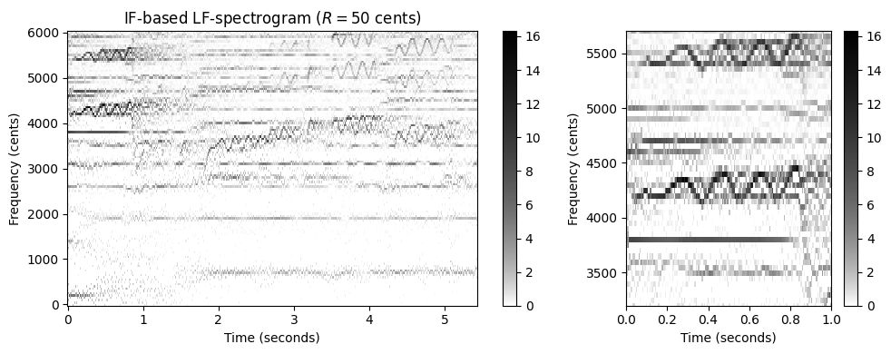
- 다음 그림에서는 \(R=10\) 센트의 해상도를 사용하는 IF 기반 로그 주파수 스펙트로그램을 보여준다. 이 높은 주파수 해상도에서도 빈(empty) 주파수 빈으로 인한 아티팩트는 거의 보이지 않는다.
R = 10
Y_LF_IF_bin, F_coef, F_coef_cents = compute_y_lf_if_bin(X, Fs, N, H, R=R,
F_min=F_min, F_max=F_max, gamma=1)
fig, ax = plt.subplots(1, 2, gridspec_kw={'width_ratios': [2, 1]}, figsize=figsize)
plot_matrix(Y_LF_IF_bin, Fs=Fs/H, F_coef=F_coef_cents, ax=[ax[0]], ylabel='Frequency (cents)',
title='IF-based LF-spectrogram ($R = %0.0f$ cents)'%R, colorbar=True, cmap=cmap);
plot_matrix(Y_LF_IF_bin, Fs=Fs/H, F_coef=F_coef_cents, ax=[ax[1]], ylabel='Frequency (cents)',
title='', colorbar=True, cmap=cmap);
ax[1].set_xlim(xlim_zoom)
ax[1].set_ylim(ylim_zoom_cents)
plt.tight_layout()C:\Users\JHCho\AppData\Local\Temp\ipykernel_15196\3605094473.py:23: RuntimeWarning: divide by zero encountered in log2
bin_index = np.floor((1200 / R) * np.log2(F / F_ref) + 0.5).astype(np.int64)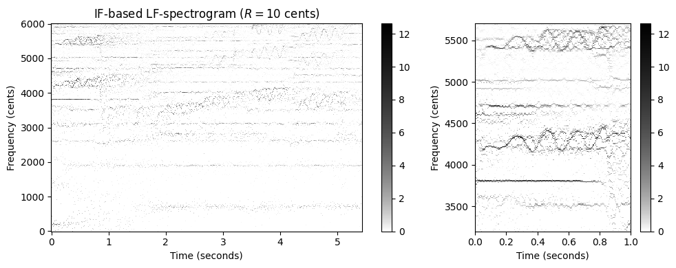
고조파 합산 (Harmonic Summation)
음악 톤과 같은 소리 이벤트는 (대략) 기본 주파수의 정수배인 고조파와 함께 기본 주파수와 연관되어 있다. 따라서 녹음된 멜로디의 스펙트로그램 표현은 일반적으로 서로 위에 쌓인 주파수 궤적의 전체 계열을 나타낸다. 크로마 시간-주파수 패턴의 여러 모양을 활용하여 스펙트로그램 표현을 개선할 수 있다.
방법은 고조파 합산(harmonic summation)이라고도 하는 기술로, 적절하게 가중된 합계를 형성하여 주파수와 해당 고조파를 공동으로 고려하는 것이다.
\(H\in\mathbb{N}\)를 합계에서 고려할 고조파 수라고 하자. 그런 다음 스펙트로그램 표현 \(\mathcal{Y}\)가 주어지면 다음을 설정하여 고조파 합 스펙트로그램 \(\tilde{\mathcal{Y}}\)를 정의한다. \[\tilde{\mathcal{Y}}(n,k) := \sum_{h=1}^{H} \alpha^{h-1} \cdot \mathcal{Y}(n,k\cdot h)\] for \(n,k\in\mathbb{Z}\) (\(\mathcal{Y}\)가 주파수 방향에서 적절하게 제로-패딩 되어 있다고 가정)
합계에서 고조파는 가중 매개변수 \(\alpha \in [0, 1]\)를 사용하여 지수(exponentially)가중 될 수 있다.
def harmonic_summation(Y, num_harm=10, alpha=1.0):
"""Harmonic summation for spectrogram [FMP, Eq. (8.54)]
Args:
Y (np.ndarray): Magnitude spectrogram
num_harm (int): Number of harmonics (Default value = 10)
alpha (float): Weighting parameter (Default value = 1.0)
Returns:
Y_HS (np.ndarray): Spectrogram after harmonic summation
"""
Y_HS = np.zeros(Y.shape)
Y_zero_pad = np.vstack((Y, np.zeros((Y.shape[0]*num_harm, Y.shape[1]))))
K = Y.shape[0]
for k in range(K):
harm_idx = np.arange(1, num_harm+1)*(k)
weights = alpha ** (np.arange(1, num_harm+1) - 1).reshape(-1, 1)
Y_HS[k, :] = (Y_zero_pad[harm_idx, :] * weights).sum(axis=0)
return Y_HSY_HS = harmonic_summation(Y, num_harm=10)
fig, ax = plt.subplots(1, 2, gridspec_kw={'width_ratios': [2, 1]}, figsize=figsize)
plot_matrix(Y_HS, Fs=Fs/H, Fs_F=N/Fs, ax=[ax[0]], title='Spectrogram after harmonic summation', colorbar=True, cmap=cmap);
ax[0].set_ylim([0, 5000])
plot_matrix(Y_HS, Fs=Fs/H, Fs_F=N/Fs, ax=[ax[1]], title='', colorbar=True, cmap=cmap);
ax[1].set_ylim(ylim_zoom)
ax[1].set_xlim(xlim_zoom)
plt.tight_layout()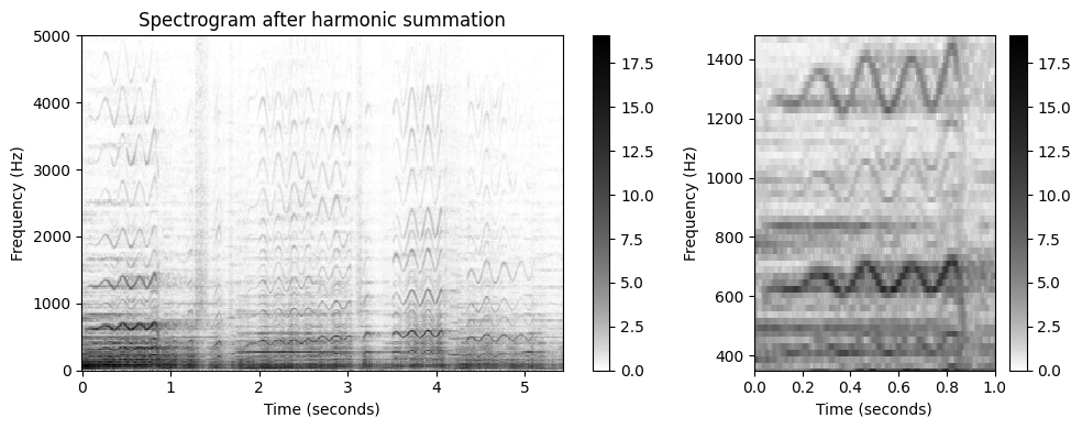
돌출 표현
\(\mathcal{Y}_\mathrm{LF}\) 또는 \(\mathcal{Y}_\mathrm{LF}^\mathrm{IF}\)와 같은 로그 주파수 스펙트로그램 표현에 유사한 구조를 적용할 수 있다.
단, 이 경우 고조파 합산의 수정이 필요하다. 특히, 로그 주파수 영역에서 작업할 때 주파수와 그것의 고조파 간의 관계는 곱셈이 아니라 덧셈이다. 예를 들어, 로그 주파수 스펙트로그램 \(\mathcal{Y}_\mathrm{LF}^\mathrm{IF}\)의 경우 고조파 합계 버전 \(\mathcal{Z}:=\tilde{ \mathcal{Y}}_\mathrm{LF}^\mathrm{IF}\)를 다음과 같이 설정하여 얻는다. \[\mathcal{Z}(n,b) := \sum_{h=1}^{H} \alpha^{h-1} \cdot \mathcal{Y}_\mathrm{LF}^\mathrm{ IF}\left(n,b+ \left\lfloor \frac{1200}{R}\log_2(h)\right\rfloor\right)\]
톤 주파수 성분의 돌출성(salience)을 강조하여 \(\mathcal{Z}\)는 돌출(salience) 표현이라고도 한다.
다음 코드 셀은 로그 주파수 표현을 위한 고조파 합계를 구현한다.
def harmonic_summation_lf(Y_LF_bin, R, num_harm=10, alpha=1.0):
"""Harmonic summation for log-frequency spectrogram [FMP, Eq. (8.55)]
Args:
Y_LF_bin (np.ndarray): Log-frequency spectrogram
R (float): Frequency resolution in cents
num_harm (int): Number of harmonics (Default value = 10)
alpha (float): Weighting parameter (Default value = 1.0)
Returns:
Y_LF_bin_HS (np.ndarray): Log-frequency spectrogram after harmonic summation
"""
Y_LF_bin_HS = np.zeros(Y_LF_bin.shape)
pad_len = int(np.floor(np.log2(num_harm) * 1200 / R))
Y_LF_bin_zero_pad = np.vstack((Y_LF_bin, np.zeros((pad_len, Y_LF_bin.shape[1]))))
B = Y_LF_bin.shape[0]
for b in range(B):
harmonics = np.arange(1, num_harm+1)
harm_idx = b + np.floor(np.log2(harmonics) * 1200 / R).astype(np.int64)
weights = alpha ** (np.arange(1, num_harm+1) - 1).reshape(-1, 1)
Y_LF_bin_HS[b, :] = (Y_LF_bin_zero_pad[harm_idx, :] * weights).sum(axis=0)
return Y_LF_bin_HSY_LF_IF_bin_HS = harmonic_summation_lf(Y_LF_IF_bin, num_harm=10, R=R)
fig, ax = plt.subplots(1, 2, gridspec_kw={'width_ratios': [2, 1]}, figsize=figsize)
plot_matrix(Y_LF_IF_bin_HS, Fs=Fs/H, F_coef=F_coef_cents, ax=[ax[0]], ylabel='Frequency (cents)',
title='IF-based LF-spectrogram after harmonic summation', colorbar=True, cmap=cmap);
plot_matrix(Y_LF_IF_bin_HS, Fs=Fs/H, F_coef=F_coef_cents, ax=[ax[1]], ylabel='Frequency (cents)',
title='', colorbar=True, cmap=cmap);
ax[1].set_xlim(xlim_zoom)
ax[1].set_ylim(ylim_zoom_cents)
plt.tight_layout()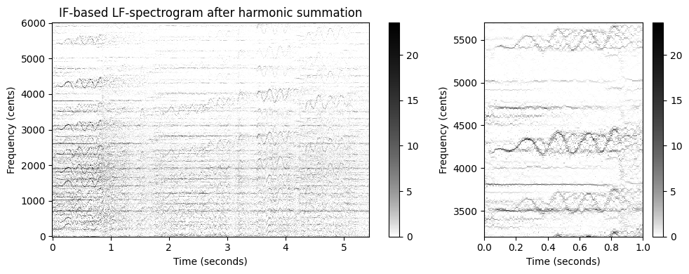
시각화를 보면 고조파 합산의 효과가 크지 않은 것 처럼 보인다. 최종 결과에 상당한 영향을 미칠 수 있는 많은 매개 변수가 있다. 특히, IF 기반 선명화(sharpening)와 결합된 높은 주파수 해상도는 고조파 관련 빈에서 작은 편차로 인해 고조파 합산에 문제를 일으킬 수 있다.
고조파 합산의 견고성을 높이는 간단한 방법은 주파수 축을 따라 스무딩(smoothing) 단계를 도입하는 것이다. 다음 그림에 표시된 대로 이 단계는 결과 돌출 표현에 상당한 영향을 미칠 수 있다.
다음 코드 셀은 최종 돌출 표현을 계산하기 위한 구현을 제공하여 전체 절차를 요약한다.
def compute_salience_rep(x, Fs, N, H, R, F_min=55.0, F_max=1760.0, num_harm=10, freq_smooth_len=11, alpha=1.0,
gamma=0.0):
"""Salience representation [FMP, Eq. (8.56)]
Args:
x (np.ndarray): Audio signal
Fs (scalar): Sampling frequency
N (int): Window length in samples
H (int): Hopsize in samples
R (float): Frequency resolution in cents
F_min (float): Lower frequency bound (reference frequency) (Default value = 55.0)
F_max (float): Upper frequency bound (Default value = 1760.0)
num_harm (int): Number of harmonics (Default value = 10)
freq_smooth_len (int): Filter length for vertical smoothing (Default value = 11)
alpha (float): Weighting parameter (Default value = 1.0)
gamma (float): Logarithmic compression factor (Default value = 0.0)
Returns:
Z (np.ndarray): Salience representation
F_coef_hertz (np.ndarray): Frequency axis in Hz
F_coef_cents (np.ndarray): Frequency axis in cents
"""
X = librosa.stft(x, n_fft=N, hop_length=H, win_length=N, pad_mode='constant')
Y_LF_IF_bin, F_coef_hertz, F_coef_cents = compute_y_lf_if_bin(X, Fs, N, H, R, F_min, F_max, gamma=gamma)
# smoothing
Y_LF_IF_bin = ndimage.convolve1d(Y_LF_IF_bin, np.hanning(freq_smooth_len), axis=0, mode='constant')
Z = harmonic_summation_lf(Y_LF_IF_bin, R=R, num_harm=num_harm, alpha=alpha)
return Z, F_coef_hertz, F_coef_centsZ, F_coef_hertz, F_coef_cents = compute_salience_rep(x, Fs, N=1024, H=128, R=10,
num_harm=10, freq_smooth_len=11, alpha=1, gamma=1)
fig, ax = plt.subplots(1, 2, gridspec_kw={'width_ratios': [2, 1]}, figsize=figsize)
plot_matrix(Z, Fs=Fs/H, F_coef=F_coef_cents, ax=[ax[0]], ylabel='Frequency (cents)',
title='Salience respresentation', colorbar=True, cmap=cmap);
plot_matrix(Z, Fs=Fs/H, F_coef=F_coef_cents, ax=[ax[1]], ylabel='Frequency (cents)',
title='', colorbar=True, cmap=cmap);
ax[1].set_xlim(xlim_zoom)
ax[1].set_ylim(ylim_zoom_cents)
plt.tight_layout()C:\Users\JHCho\AppData\Local\Temp\ipykernel_15196\3605094473.py:23: RuntimeWarning: divide by zero encountered in log2
bin_index = np.floor((1200 / R) * np.log2(F / F_ref) + 0.5).astype(np.int64)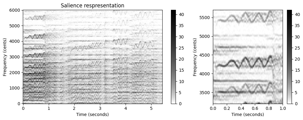
이 그림에서 볼 수 있듯이 합산 프로세스는 지배적인 톤 구성 요소를 증폭하는 반면 순간 주파수 추정에 의해 도입된 노이즈와 같은 아티팩트가 감쇠된다.
단, 단점은 프로세스가 특히 스펙트로그램의 낮은 주파수 범위에 나타나는 고스트(ghost) 요소를 생성한다는 것이다(예: 오른쪽 플롯에서 주파수 \(3500\) 센트 주변의 비브라토 참조). 그러나 이것은 지배 주파수 궤적(predominant frequency trajectories)만을 찾는 경우에는 큰 문제가 되지 않는다.
요약하면, 돌출(salience) 표현 \(\mathcal{Z}\)의 구성은 몇 가지 가정과 관찰에 의해 동기가 부여된다.
- 첫째, 로그 주파수 비닝은 주파수의 로그 인식과 음 피치의 음악적 개념을 설명한다.
- 둘째, 순간 주파수를 사용하면 주파수 추정의 정확도가 향상된다.
- 셋째, 고조파 합산은 규칙적인 간격의 주파수 성분을 증폭시킨다. 이것은 톤의 에너지가 기본 주파수에 포함되어 있을 뿐만 아니라 전체 고조파 스펙트럼에 퍼져 있다는 사실을 설명한다.
게다가, 우리는 고조파 합산 이전의 추가 스무딩 단계가 최종 돌출 표현에서 상당한 개선을 가져올 수 있음을 확인했다.
일반적으로 고해상도로 샘플링된 데이터에 로컬 연산을 적용할 때 데이터의 작은 편차나 이상값은 상당한 성능 저하로 이어질 수 있다. 이러한 상황에서 추가 필터링 단계(예: 가우스 커널 또는 중앙값 필터링을 사용한 컨볼루션)는 일부 문제를 완화하는 데 도움이 될 수 있다.
위에서 본 경우 스무딩은 고조파 합산을 적용하기 전에 주파수 빈의 작은 편차의 균형을 맞추는 데 도움이 되었다. 노벨티 기반 경계 감지와 관련하여 유사한 전략을 적용했다. 여기서 노벨티 함수 \(\Delta_\mathrm{Structure}\)를 계산하기 위해서는 연속되는 특징들 간의 지역적 차이를 계산하기 전에 추가적인 필터링이 유리했다.
기본 주파수 추적 (Fundamental Frequency Tracking)
주파수 궤적 (Frequency Trajectory)
일반적으로 멜로디(melody)는 일관된 개체를 형성하고 특정 음악적 아이디어를 표현하는 음악 톤의 선형적 연속(succession)으로 정의될 수 있다. 음악 처리의 다른 많은 개념과 마찬가지로 멜로디의 개념은 다소 모호하다. 이 포스트에서는 음악이 오디오 녹음의 형태로 제공되는 시나리오(심볼릭 음악 표현이 아님)를 고려한다.
또한 음의 순서를 추정하는 것이 아니라 음의 피치에 해당하는 주파수 값의 순서를 결정하는 것이 목표이다. 연속적인 주파수 글라이드(glides) 및 변조(modulation)를 캡처할 수 있는 시간 경과에 따른 이러한 주파수 경로를 주파수 궤적(trajectory) 이라고 한다. 특히 멜로디 음표의 기본 주파수 값(F0 값이라고도 함)에 관심이 있다. 그 결과의 궤적은 F0-궤적이라고도 한다.
수학적으로 F0-궤적을 다음의 함수로 모델링한다. \[\eta:\mathbb{R}\to\mathbb{R}\cup\{\ast\}\]
- 이는 각 시점 \(t\in\mathbb{R}\)(초 단위)에 주파수 값 \(\eta(t)\in\mathbb{R}\)(Hertz 단위) 또는 기호 \(\eta(n)=\ast\)를 할당한다.
- \(\eta(t)=\ast\)은 이 시점에서 멜로디 성분에 해당하는 F0 값이 없다는 뜻이다.
예시로 위에서 봤던 “Der Freischütz” - Carl Maria von Weber를 보자. 악보 표현에서 주요 멜로디는 가사와 함께 표시되어 있다. 소프라노 가수의 퍼포먼스에서 멜로디는 F0-값의 궤적에 해당한다. 표시된 기호적 표현과 반대로, 몇몇 음은 부드럽게 연결되어 있다. 더욱이 비브라토에 따른 뚜렷한 주파수 변조를 되려 관찰 할 수 있다.
ipd.display(Image(path_img+"FMP_C8_F10a.png", width=300))
ipd.display(Audio(path_data+"FMP_C8_F10_Weber_Freischuetz-06_FreiDi-35-40.wav"))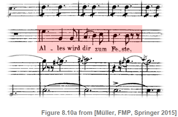
- 다음 그림에서는 가수의 F0-궤적(주석 파일에서 읽음)을 시각화한다. 하나는 선형 주파수 축(Hertz로 주어짐)과 로그 주파수 축(참고 주파수\(\omega_\mathrm{ref}=55~\mathrm{Hz}\) 에 상대적인 센트로 주어짐)으로 한 번 표시된다.
def hz_to_cents(F, F_ref=55.0):
"""Converts frequency in Hz to cents
Args:
F (float or np.ndarray): Frequency value in Hz
F_ref (float): Reference frequency in Hz (Default value = 55.0)
Returns:
F_cent (float or np.ndarray): Frequency in cents
"""
F_cent = 1200 * np.log2(F / F_ref)
return F_cent
def cents_to_hz(F_cent, F_ref=55.0):
"""Converts frequency in cents to Hz
Args:
F_cent (float or np.ndarray): Frequency in cents
F_ref (float): Reference frequency in Hz (Default value = 55.0)
Returns:
F (float or np.ndarray): Frequency in Hz
"""
F = F_ref * 2 ** (F_cent / 1200)
return F# Load audio
fn_wav = 'FMP_C8_F10_Weber_Freischuetz-06_FreiDi-35-40.wav'
x, Fs = librosa.load(path_data+fn_wav)
x_duration = len(x)/Fs
ipd.Audio(x, rate=Fs)
# Read in the F0 trajectory
fn_traj = 'FMP_C8_F10_Weber_Freischuetz-06_FreiDi-35-40_F0-user-Book.csv'
traj_df = pd.read_csv(path_data+fn_traj,sep=';', keep_default_na=False, header=0)
traj = traj_df.values
fig, ax = plt.subplots(3, 1, gridspec_kw={'height_ratios': [1, 2, 2]}, figsize=(6,5))
plot_signal(x, Fs, ax=ax[0], xlabel='');
ax[0].set_ylim((-1,1));
ax[0].set_ylabel('Amplitude')
ax[0].set_xlabel('Time (seconds)')
traj_plot = traj[traj[:, 1]>0]
ax[1].plot(traj_plot[:, 0], traj_plot[:, 1], color='r', markersize=4, marker='.', linestyle='');
ax[1].set_ylim((55,880));
ax[1].set_yticks([55, 220, 440, 660, 880])
ax[1].set_xlim((0, x_duration));
ax[1].set_ylabel('Frequency (Hertz)')
ax[1].set_xlabel('Time (seconds)')
plt.tight_layout()
ax[2].plot(traj_plot[:, 0], hz_to_cents(traj_plot[:, 1]), color='r', markersize=4, marker='.', linestyle='');
ax[2].set_ylim((2400, 4800));
ax[2].set_yticks([2400, 3600, 4800])
ax[2].set_xlim((0, x_duration));
plt.xlabel('Time (seconds)')
ax[2].set_ylabel('Frequency (Cents)')
plt.tight_layout()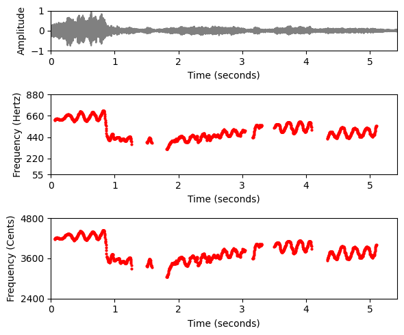
Sonification
def sonify_trajectory_with_sinusoid(traj, audio_len, Fs=22050, amplitude=0.3, smooth_len=11):
"""Sonification of trajectory with sinusoidal
Args:
traj (np.ndarray): F0 trajectory (time in seconds, frequency in Hz)
audio_len (int): Desired audio length in samples
Fs (scalar): Sampling rate (Default value = 22050)
amplitude (float): Amplitude (Default value = 0.3)
smooth_len (int): Length of amplitude smoothing filter (Default value = 11)
Returns:
x_soni (np.ndarray): Sonification
"""
# unit confidence if not specified
if traj.shape[1] < 3:
confidence = np.zeros(traj.shape[0])
confidence[traj[:, 1] > 0] = amplitude
else:
confidence = traj[:, 2]
# initialize
x_soni = np.zeros(audio_len)
amplitude_mod = np.zeros(audio_len)
# Computation of hop size
# sine_len = int(2 ** np.round(np.log(traj[1, 0]*Fs) / np.log(2)))
sine_len = int(traj[1, 0] * Fs)
t = np.arange(0, sine_len) / Fs
phase = 0
# loop over all F0 values, insure continuous phase
for idx in np.arange(0, traj.shape[0]):
cur_f = traj[idx, 1]
cur_amp = confidence[idx]
if cur_f == 0:
phase = 0
continue
cur_soni = np.sin(2*np.pi*(cur_f*t+phase))
diff = np.maximum(0, (idx+1)*sine_len - len(x_soni))
if diff > 0:
x_soni[idx * sine_len:(idx + 1) * sine_len - diff] = cur_soni[:-diff]
amplitude_mod[idx * sine_len:(idx + 1) * sine_len - diff] = cur_amp
else:
x_soni[idx*sine_len:(idx+1)*sine_len-diff] = cur_soni
amplitude_mod[idx*sine_len:(idx+1)*sine_len-diff] = cur_amp
phase += cur_f * sine_len / Fs
phase -= 2 * np.round(phase/2)
# filter amplitudes to avoid transients
amplitude_mod = np.convolve(amplitude_mod, np.hanning(smooth_len)/np.sum(np.hanning(smooth_len)), 'same')
x_soni = x_soni * amplitude_mod
return x_sonix_traj_mono = sonify_trajectory_with_sinusoid(traj, len(x), Fs, smooth_len=11, amplitude=0.6)
# left: x, right: sonification
x_traj_stereo = np.vstack((x.reshape(1,-1), x_traj_mono.reshape(1,-1)))
print('F0 sonification (mono)')
ipd.display(Audio(x_traj_mono, rate=Fs))
print('F0 sonification superimposed with original recording (mono)')
ipd.display(Audio( (x_traj_mono+x)/2, rate=Fs))
#print('F0 sonification (right channel), original recording (left channel)')
#ipd.display(Audio(x_traj_stereo, rate=Fs))F0 sonification (mono)F0 sonification superimposed with original recording (mono)돌출성 기반 주파수 추적
종종 메인 멜로디는 주어진 오디오 신호에서 가장 강한 하모닉 소스(harmonic source)라는 의미에서 지배적(dominant)이다.
리드 싱어나 리드 악기가 주로 멜로디를 연주하는 음악으로 제한해서 보기로 한다. 특히 하나의 음원에 연관될 수 있는 멜로디 라인은 한 번에 하나뿐이라고 가정한다.
이 시나리오에서 메인 멜로디를 추출하기 위한 간단한 방법은 각 시간 프레임에서 가장 강한 고조파 주파수 성분을 찾는 것이다. 돌출(salience) 표현을 설계하는 목적은 강한 고조파 성분을 향상시키는 것이었다. 따라서 멜로디 추출을 위한 첫 번째 전략은 돌출 표현의 프레임별 최대값을 고려하는 것이다.
다음에서 \(\mathcal{Z}\)는 \(\mathcal{Z}(n,b)\in\mathbb{R}\) 항목을 포함하는 돌출 표현을 나타낸다고 하자. 여기서 \(n\in[1:N]\) 프레임 인덱스를 나타내고, \(b\in[1:B]\)는 빈(bin) 인덱스를 나타낸다.
def visualize_salience_traj_constraints(Z, T_coef, F_coef_cents, F_ref=55.0, colorbar=True, cmap='gray_r',
figsize=(7, 4), traj=None, constraint_region=None, ax=None):
"""Visualize salience representation with optional F0-trajectory and constraint regions
Args:
Z: Salience representation
T_coef: Time axis
F_coef_cents: Frequency axis in cents
F_ref: Reference frequency (Default value = 55.0)
colorbar: Show or hide colorbar (Default value = True)
cmap: Color map (Default value = 'gray_r')
figsize: Figure size (Default value = (7, 4))
traj: F0 trajectory (time in seconds, frequency in Hz) (Default value = None)
constraint_region: Constraint regions, row-format: (t_start_sec, t_end_sec, f_start_hz, f_end,hz)
(Default value = None)
ax: Handle to existing axis (Default value = None)
Returns:
fig: Handle to figure
ax: Handle to cent axis
ax_f: Handle to frequency axis
"""
fig = None
if ax is None:
fig, ax = plt.subplots(1, 1, figsize=figsize)
sal = ax.imshow(Z, extent=[T_coef[0], T_coef[-1], F_coef_cents[0], F_coef_cents[-1]],
cmap=cmap, origin='lower', aspect='auto', interpolation='nearest')
y_ticklabels_left = np.arange(F_coef_cents[0], F_coef_cents[-1]+1, 1200)
ax.set_yticks(y_ticklabels_left)
ax.set_yticklabels(y_ticklabels_left)
ax.set_ylabel('Frequency (Cents)')
if colorbar:
plt.colorbar(sal, ax=ax, pad=0.1)
ax_f = ax.twinx() # instantiate a second axes that shares the same y-axis
ax_f.set_yticks(y_ticklabels_left - F_coef_cents[0])
y_ticklabels_right = cents_to_hz(y_ticklabels_left, F_ref).astype(int)
ax_f.set_yticklabels(y_ticklabels_right)
ax_f.set_ylabel('Frequency (Hz)')
# plot contour
if traj is not None:
traj_plot = traj[traj[:, 1] > 0, :]
traj_plot[:, 1] = hz_to_cents(traj_plot[:, 1], F_ref)
ax.plot(traj_plot[:, 0], traj_plot[:, 1], color='r', markersize=4, marker='.', linestyle='')
# plot constraint regions
if constraint_region is not None:
for row in constraint_region:
t_start = row[0] # sec
t_end = row[1] # sec
f_start = row[2] # Hz
f_end = row[3] # Hz
ax.add_patch(matplotlib.patches.Rectangle((
t_start, hz_to_cents(f_start, F_ref)), width=t_end-t_start,
height=hz_to_cents(f_end, F_ref)-hz_to_cents(f_start, F_ref),
fill=False, edgecolor='k', linewidth=3, zorder=2))
ax.set_xlabel('Time (seconds)')
if fig is not None:
plt.tight_layout()
return fig, ax, ax_f# Computation of salience representation
N = 1024
H = 128
R = 10
F_min = 55.0
F_max = 1760.0
num_harm = 8
freq_smooth_len = 11
alpha = 0.9
gamma = 0.1
Z, F_coef_hertz, F_coef_cents = compute_salience_rep(x, Fs, N=N, H=H, R=R,
F_min=F_min, F_max=F_max, num_harm=num_harm,
freq_smooth_len=freq_smooth_len, alpha=alpha, gamma=gamma)
T_coef = (np.arange(Z.shape[1]) * H) / Fs
# Visualization
figsize = (10,3)
cmap = compressed_gray_cmap(alpha=5)
visualize_salience_traj_constraints(Z, T_coef, F_coef_cents, F_ref=F_min, figsize=figsize, cmap=cmap,
colorbar=True, ax=None)
plt.show()C:\Users\JHCho\AppData\Local\Temp\ipykernel_15196\3605094473.py:23: RuntimeWarning: divide by zero encountered in log2
bin_index = np.floor((1200 / R) * np.log2(F / F_ref) + 0.5).astype(np.int64)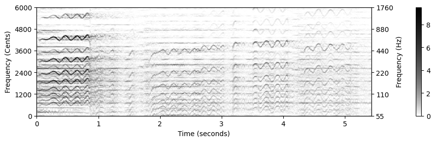
이산(discrete) 설정에서 주파수 궤적은 각 프레임 인덱스 \(n\in[1:N]\) 에 할당되는 \(\eta:[1:N]\to[1:B]\cup\{\ast\}\) 함수로 정의된다. 이 때 각 프레임 인덱스는 빈 인덱스 \(\eta(n)\in[1:B]\) 또는 기호 \(\eta(n)=\ast\)이다.
각 프레임에 대해 \(\mathcal{Z}\)의 빈 인덱스를 최대화하면, \(\eta^\mathrm{max}(n):= \underset{b\in[1:B]}{\mathrm{argmax}}\,\, \mathcal{Z}(n,b)\)로 정의된 주파수 궤적 \(\eta^\mathrm{max}\)를 얻는다.
다음 그림은 간단한 F0 궤적 추적 절차를 보여준다. 다수의 이상값과 시간적 불연속성을 관찰할 수 있다. 이 방법은 멜로디가 실제로 존재하는지 여부에 관계없이 각 시간 프레임에 F0 값을 할당한다.
# Frequency trajectory via maximization
index_max = np.argmax(Z, axis=0)
traj = np.hstack((T_coef.reshape(-1, 1), F_coef_hertz[index_max].reshape(-1, 1)))
# Visualization
figsize = (10,3)
cmap = compressed_gray_cmap(alpha=5)
visualize_salience_traj_constraints(Z, T_coef, F_coef_cents, F_ref=F_min, figsize=figsize, cmap=cmap,
colorbar=True, traj=traj, ax=None)
plt.show()
# Sonification
x_traj_mono = sonify_trajectory_with_sinusoid(traj, len(x), Fs, smooth_len=11)
x_traj_stereo = np.vstack((x.reshape(1,-1), x_traj_mono.reshape(1,-1)))
ipd.display(Audio(x_traj_mono, rate=Fs))
#print('F0 sonification (right channel), original recording (left channel)')
#ipd.display(Audio(x_traj_stereo, rate=Fs))
연속성 제약 (Continuity Constraints)
시간적 맥락을 고려하지 않고 순전히 프레임 방식으로 주파수 궤적을 계산하면 로컬 불연속성 및 무작위 점프가 발생할 수 있다. 실제로 멜로디의 주파수 궤적은 훨씬 더 구조화되어 있다. 일반적으로 음 전환 사이에 간헐적으로 점프하면서 시간이 지남에 따라 천천히 변경된다.
이제 시간적 유연성(temporal flexibility)(가능한 점프를 설명하기 위해)과 시간적 연속성(temporal continuity)(스무스한(smoothness) 속성을 설명하기 위해)이라는 두 가지 상충되는 조건의 균형을 맞출 수 있는 절차에 대해 논의한다.
\(\mathcal{Z}\)를 \(N\) 시간 프레임과 \(B\) 주파수 빈으로 구성된 돌출(salience) 표현이라고 하자. \(\mathcal{Z}(n,b)\) 값은 시간 \(n\in[1:N]\)에 빈 \(b\in[1:B]\)과 관련된 주파수가 지배적인 음조에 속할 가능도(likelihood)를 나타내는 점수로 간주될 수 있다
또한, \(T\in\mathbb{R}^{B\times B}\)를 전이(transition) 행렬이라고 하자. 여기서 항목 \(T(b,c)\in\mathbb{R}\)가 시간 프레임 \(n\in[1:N-1]\)의 빈 \(b\in[1:B]\)에서 시간 프레임 \(n\in[1:N-1]\)의 빈 \(c\in[1:B]\)로 이동할 가능도를 나타낸다.
이러한 전이 행렬을 정의하는 방법에는 여러 가지가 있다. \(T\)가 가까운 빈(예: \(|b-c|\)가 작을 때 \(\mathbf{T}(b,c)\approx 1\)) 사이의 전이를 선호하고 멀리 떨어진 빈 사이의 전이에는 페널티를 준다. (예: \(|b-c|\)가 클 때 \(\mathbf{T}(b,c)\approx \delta\) , 작은 양수값 \(\delta>0\)). 예를 들어, 큰 편차에는 무관심하면서 \(\pm 50\) 센트까지의 작은 변동은 선호할 수 있다.
다음 코드 셀에서 이러한 요구 사항을 충족하는 전이 행렬 \(T\)를 정의한다.
def define_transition_matrix(B, tol=0, score_low=0.01, score_high=1.0):
"""Generate transition matrix
Args:
B (int): Number of bins
tol (int): Tolerance parameter for transition matrix (Default value = 0)
score_low (float): Score (low) for transition matrix (Default value = 0.01)
score_high (float): Score (high) for transition matrix (Default value = 1.0)
Returns:
T (np.ndarray): Transition matrix
"""
col = np.ones((B,)) * score_low
col[0:tol+1] = np.ones((tol+1, )) * score_high
T = scipy.linalg.toeplitz(col)
return T# Compute transition matrix
T = define_transition_matrix(B=51, tol=5)
# Plot
colorList = np.array([[1,0.9,0.9,1],[0,0,0,1]])
cmap = ListedColormap(colorList)
plt.figure(figsize=(4,3))
im = plt.imshow(T, origin='lower', cmap=cmap)
plt.title('Transition matrix')
plt.xlabel('Bin index')
plt.ylabel('Bin index')
ax_cb = plt.colorbar(im)
ax_cb.set_ticks(np.array([0.25, 0.75]))
ax_cb.set_ticklabels(np.array([np.min(T), np.max(T)])) 
돌출 표현 \(\mathcal{Z}\)와 전이 우도(transition likelihood) 행렬 \(\mathbf{T}\)가 주어지면 각 궤적 \(\eta:[1:N]\to[1:B]\)에 총점(total score) \(\sigma(\eta)\)을 연결할 수 있다. \[\sigma(\eta) := \mathcal{Z}(1,\eta(1)) \cdot \prod_{n=2}^{N} \Big(\mathbf{T}(\eta(n- 1),\eta(n))\cdot \mathcal{Z}(n,\eta(n))\Big)\]
원하는 궤적 \(\eta^\mathrm{DP}\)는 점수 최대화 궤적으로 정의된다. \[\eta^\mathrm{DP} := \underset{\eta}{\mathrm{argmax}} \,\, \sigma(\eta)\]
동적 프로그래밍(Viterbi 알고리즘과 유사)을 통해 최대 총점을 계산할 수 있다. 또한 적절한 역추적 절차를 적용하여 궤적 \(\eta^\mathrm{DP}\)를 얻을 수 있다.
많은 요소의 곱을 계산할 때 수치적 불안정성(예: 곱이 0에 접근하는 언더플로(underflow) 문제)에 자주 직면하게 된다. 따라서 실제로는 곱이 합이 되는 로그 도메인에서 최적화 접근 방식을 구현해야 한다. 이러한 접근 방식은 다음 구현에서 사용된다.
def compute_trajectory_dp(Z, T):
"""Trajectory tracking using dynamic programming
Args:
Z: Salience representation
T: Transisition matrix
Returns:
eta_DP (np.ndarray): Trajectory indices
"""
B, N = Z.shape
eps_machine = np.finfo(np.float32).eps
Z_log = np.log(Z + eps_machine)
T_log = np.log(T + eps_machine)
E = np.zeros((B, N))
D = np.zeros((B, N))
D[:, 0] = Z_log[:, 0]
for n in np.arange(1, N):
for b in np.arange(0, B):
D[b, n] = np.max(T_log[b, :] + D[:, n-1]) + Z_log[b, n]
E[b, n-1] = np.argmax(T_log[b, :] + D[:, n-1])
# backtracking
eta_DP = np.zeros(N)
eta_DP[N-1] = int(np.argmax(D[:, N-1]))
for n in np.arange(N-2, -1, -1):
eta_DP[n] = E[int(eta_DP[n+1]), n]
return eta_DP.astype(np.int64)# Frequency trajectory via DP-based optimization
B, N = Z.shape
T = define_transition_matrix(B, tol=5)
index_DP = compute_trajectory_dp(Z, T)
traj = np.hstack((T_coef.reshape(-1, 1), F_coef_hertz[index_DP].reshape(-1, 1)))
# Visualization
figsize = (10,3)
cmap = compressed_gray_cmap(alpha=10)
visualize_salience_traj_constraints(Z, T_coef, F_coef_cents, F_ref=F_min,
figsize=figsize, cmap=cmap,
colorbar=True, traj=traj, ax=None)
plt.show()
# Sonification
x_traj_mono = sonify_trajectory_with_sinusoid(traj, len(x), Fs, smooth_len=11)
x_traj_stereo = np.vstack((x.reshape(1,-1), x_traj_mono.reshape(1,-1)))
ipd.display(Audio(x_traj_mono, rate=Fs))
#print('F0 sonification (right channel), original recording (left channel)')
#ipd.display(Audio(x_traj_stereo, rate=Fs))
- 그림은 Freischütz 예의 결과를 보여준다. 단순힌 최대화 접근 방식과 비교해서, 전이 우도에 의해 도입된 연속성 제약 덕분에 대부분의 이상값이 제거되었다. 단, 반주가 멜로디보다 강한 조성 성분을 나타낼 경우 여전히 트래킹 오류가 발생한다.
악보 정보 제약 (Score-Informed Constraints)
연속성 제약을 통합하는 것 외에 또 다른 전략은 F0-추적 프로세스를 지원하기 위해 멜로디 진행에 대한 추가 음악적 지식을 활용하는 것이다. 예를 들어, 가수의 음역(소프라노, 알토, 테너, 베이스)을 알면 예상되는 F0 값의 검색 범위를 좁힐 수 있다. 또는 멜로디가 실제로 존재하는 경우와 존재하지 않는 경우에 대한 정보를 가지고 비멜로디 프레임에 대해 모든 F0 값을 ‘\(\ast\)’ 기호로 설정할 수 있다.
보다 일반적으로, 위에서 설명한 추가 지식을 사용하여 시간-주파수 평면 내의 제약 영역(constraint regions)을 정의할 수 있다. 그런 다음 이러한 지정된 영역에서만 F0 추적이 수행된다.
이러한 접근 방식의 예로, 주어진 음악 녹음의 기초가 되는 악보 표현의 가용성을 가정하는 악보 정보 절차(score-informed procedure)에 대해 논의하자. 악보에서 제공하는 추가 악기 및 음표 정보는 멜로디의 F0 궤적 추정을 도울 수 있다.
- 첫 번째 단계에서 악보와 주어진 오디오 녹음을 정렬해야 한다. 이는 수동적인 주석 프로세스에서 수행되거나 음악 동기화 기술을 사용하여 (반)자동으로 수행될 수 있다.
- 그런 다음 정렬된 악보 정보를 사용하여 멜로디에서 발생하는 음에 대한 시간-주파수 평면의 직사각형 제약 영역을 정의할 수 있다. 이러한 각 영역의 수평 위치와 너비는 음표의 물리적 시작 시간과 예상 지속 시간에 해당하는 반면, 수직 위치와 높이는 음표의 피치와 중심 주파수에서 예상되는 주파수 편차를 설명한다.
- 마지막으로, 각각의 제한 영역에 대해 위의 절차를 적용하여 음표별(notewise) 주파수 궤적을 계산할 수 있다. 음표의 제약 영역의 시간적 중첩이 없다고 가정하면, 악보 정보가 포함된 단일 궤적 \(\eta^\mathrm{Score}\)를 형성하기 위해 음표 궤적을 조합할 수 있다. \(n\in[1:N]\) 프레임이 제약 영역에 포함되지 않는 경우 \(\eta^\mathrm{Score}(n):=\ast\)를 설정한다.
다음 코드 셀에서 악보 정보 절차의 구현을 볼 수 있다.
- 제약 영역을 정의하는 데 사용되는 정렬된 악보 정보는 주석 파일로부터 읽는다.
- 악보 정보를 제약 영역으로 변환할 때 중심 주파수 주변의 주파수 방향(센트 단위로 지정)에 대한 허용 오차를 사용한다.
- 값 ‘\(\ast\)’(소위 무성 프레임을 나타냄)는 빈 인덱스
-1을 사용하여 인코딩된다.
def convert_ann_to_constraint_region(ann, tol_freq_cents=300.0):
"""Convert score annotations to constraint regions
Args:
ann (list): Score annotations [[start_time, end_time, MIDI_pitch], ...
tol_freq_cents (float): Tolerance in pitch directions specified in cents (Default value = 300.0)
Returns:
constraint_region (np.ndarray): Constraint regions
"""
tol_pitch = tol_freq_cents / 100
freq_lower = 2 ** ((ann[:, 2] - tol_pitch - 69)/12) * 440
freq_upper = 2 ** ((ann[:, 2] + tol_pitch - 69)/12) * 440
constraint_region = np.concatenate((ann[:, 0:2],
freq_lower.reshape(-1, 1),
freq_upper.reshape(-1, 1)), axis=1)
return constraint_region
def compute_trajectory_cr(Z, T_coef, F_coef_hertz, constraint_region=None,
tol=5, score_low=0.01, score_high=1.0):
"""Trajectory tracking with constraint regions
Args:
Z (np.ndarray): Salience representation
T_coef (np.ndarray): Time axis
F_coef_hertz (np.ndarray): Frequency axis in Hz
constraint_region (np.ndarray): Constraint regions, row-format: (t_start_sec, t_end_sec, f_start_hz, f_end_hz)
(Default value = None)
tol (int): Tolerance parameter for transition matrix (Default value = 5)
score_low (float): Score (low) for transition matrix (Default value = 0.01)
score_high (float): Score (high) for transition matrix (Default value = 1.0)
Returns:
eta (np.ndarray): Trajectory indices, unvoiced frames are indicated with -1
"""
# do tracking within every constraint region
if constraint_region is not None:
# initialize contour, unvoiced frames are indicated with -1
eta = np.full(len(T_coef), -1)
for row_idx in range(constraint_region.shape[0]):
t_start = constraint_region[row_idx, 0] # sec
t_end = constraint_region[row_idx, 1] # sec
f_start = constraint_region[row_idx, 2] # Hz
f_end = constraint_region[row_idx, 3] # Hz
# convert start/end values to indices
t_start_idx = np.argmin(np.abs(T_coef - t_start))
t_end_idx = np.argmin(np.abs(T_coef - t_end))
f_start_idx = np.argmin(np.abs(F_coef_hertz - f_start))
f_end_idx = np.argmin(np.abs(F_coef_hertz - f_end))
# track in salience part
cur_Z = Z[f_start_idx:f_end_idx+1, t_start_idx:t_end_idx+1]
T = define_transition_matrix(cur_Z.shape[0], tol=tol,
score_low=score_low, score_high=score_high)
cur_eta = compute_trajectory_dp(cur_Z, T)
# fill contour
eta[t_start_idx:t_end_idx+1] = f_start_idx + cur_eta
else:
T = define_transition_matrix(Z.shape[0], tol=tol, score_low=score_low, score_high=score_high)
eta = compute_trajectory_dp(Z, T)
return eta# Read score annotations and convert to constraint regions
fn_score = 'FMP_C8_F10_Weber_Freischuetz-06_FreiDi-35-40_CR-score.csv'
ann_score_df = pd.read_csv(path_data+fn_score, sep=';', keep_default_na=False, header=0)
print('Score annotations:')
ipd.display(ann_score_df)
ann_score = ann_score_df.values
constraint_region = convert_ann_to_constraint_region(ann_score, tol_freq_cents=300)
print('Constraint regions:')
print(constraint_region)Score annotations:| start_time | end_time | MIDI_pitch | |
|---|---|---|---|
| 0 | 0.0 | 0.9 | 76 |
| 1 | 0.9 | 1.6 | 68 |
| 2 | 1.6 | 1.9 | 68 |
| 3 | 1.9 | 2.6 | 69 |
| 4 | 2.6 | 3.1 | 71 |
| 5 | 3.1 | 3.4 | 73 |
| 6 | 3.4 | 4.2 | 71 |
| 7 | 4.2 | 4.8 | 71 |
Constraint regions:
[[ 0. 0.9 554.36526195 783.99087196]
[ 0.9 1.6 349.22823143 493.88330126]
[ 1.6 1.9 349.22823143 493.88330126]
[ 1.9 2.6 369.99442271 523.2511306 ]
[ 2.6 3.1 415.30469758 587.32953583]
[ 3.1 3.4 466.16376152 659.25511383]
[ 3.4 4.2 415.30469758 587.32953583]
[ 4.2 4.8 415.30469758 587.32953583]]# Frequency trajectory using constraint regions
index_CR = compute_trajectory_cr(Z, T_coef, F_coef_hertz, constraint_region, tol=5)
traj = np.hstack((T_coef.reshape(-1, 1), F_coef_hertz[index_CR].reshape(-1, 1)))
traj[index_CR==-1, 1] = 0 # set unvoiced frames to zero
# Visualization
visualize_salience_traj_constraints(Z, T_coef, F_coef_cents, F_ref=F_min, figsize=figsize, cmap=cmap,
constraint_region=constraint_region, colorbar=True, traj=traj, ax=None)
plt.show()
# Sonification
x_traj_mono = sonify_trajectory_with_sinusoid(traj, len(x), Fs, smooth_len=11)
x_traj_stereo = np.vstack((x.reshape(1,-1), x_traj_mono.reshape(1,-1)))
ipd.display(Audio(x_traj_mono, rate=Fs))
#print('F0 sonification (right channel), original recording (left channel)')
#ipd.display(Audio(x_traj_stereo, rate=Fs))
악보-정보 제약 영역이 정확하지 않은 경우(예: 동기화 부정확성 또는 악보와 오디오 녹음 간의 편차로 인해) 절차에 문제가 발생하여 주파수 궤적이 손상될 수 있다. 이러한 오류는 제약 영역을 적절하게 조정하여 수정할 수 있다.
다음 예는 결과 F0 궤적과 함께 사용자-최적화(user-optimzied) 제약 영역을 보여준다.
# Read constraint regions
fn_region = 'FMP_C8_F10_Weber_Freischuetz-06_FreiDi-35-40_CR-user.csv'
constraint_region_df = pd.read_csv(path_data+fn_region, sep=';', keep_default_na=False, header=0)
constraint_region = constraint_region_df.values
index_CR = compute_trajectory_cr(Z, T_coef, F_coef_hertz, constraint_region, tol=5)
traj = np.hstack((T_coef.reshape(-1, 1), F_coef_hertz[index_CR].reshape(-1, 1)))
traj[index_CR==-1, 1] = 0 # set unvoiced frames to zero
# Visualization
visualize_salience_traj_constraints(Z, T_coef, F_coef_cents, F_ref=F_min,
figsize=figsize, cmap=cmap,
constraint_region=constraint_region,
colorbar=True, traj=traj, ax=None)
plt.show()
# Sonification
x_traj_mono = sonify_trajectory_with_sinusoid(traj, len(x), Fs, smooth_len=11)
x_traj_stereo = np.vstack((x.reshape(1,-1), x_traj_mono.reshape(1,-1)))
ipd.display(ipd.Audio(x_traj_mono, rate=Fs))
#print('F0 sonification (right channel), original recording (left channel)')
#ipd.display(ipd.Audio(x_traj_stereo, rate=Fs))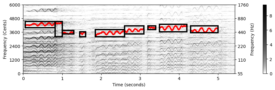
전체 과정: 예시
F0-궤적의 (제약-기반) 전체 계산 절차를 보자.
예로 Sven Bornemark의 노래 “Stop Messing With Me”의 발췌 부분에 적용한다. 발췌 부분에서 남성 가수가 드럼, 피아노, 기타 반주로 멜로디를 연주한다. 언제 가수가 노래하고, 노래하는 피치의 범위가 어떻게 되는지 인코딩하는 제약 영역이 이미 주어져있는 경우를 고려한다.
def compute_traj_from_audio(x, Fs=22050, N=1024, H=128, R=10.0, F_min=55.0, F_max=1760.0,
num_harm=10, freq_smooth_len=11, alpha=0.9, gamma=0.0,
constraint_region=None, tol=5, score_low=0.01, score_high=1.0):
"""Compute F0 contour from audio signal
Args:
x (np.ndarray): Audio signal
Fs (scalar): Sampling frequency (Default value = 22050)
N (int): Window length in samples (Default value = 1024)
H (int): Hopsize in samples (Default value = 128)
R (float): Frequency resolution in cents (Default value = 10.0)
F_min (float): Lower frequency bound (reference frequency) (Default value = 55.0)
F_max (float): Upper frequency bound (Default value = 1760.0)
num_harm (int): Number of harmonics (Default value = 10)
freq_smooth_len (int): Filter length for vertical smoothing (Default value = 11)
alpha (float): Weighting parameter for harmonics (Default value = 0.9)
gamma (float): Logarithmic compression factor (Default value = 0.0)
constraint_region (np.ndarray): Constraint regions, row-format: (t_start_sec, t_end_sec, f_start_hz, f_end,hz)
(Default value = None)
tol (int): Tolerance parameter for transition matrix (Default value = 5)
score_low (float): Score (low) for transition matrix (Default value = 0.01)
score_high (float): Score (high) for transition matrix (Default value = 1.0)
Returns:
traj (np.ndarray): F0 contour, time in seconds in 1st column, frequency in Hz in 2nd column
Z (np.ndarray): Salience representation
T_coef (np.ndarray): Time axis
F_coef_hertz (np.ndarray): Frequency axis in Hz
F_coef_cents (np.ndarray): Frequency axis in cents
"""
Z, F_coef_hertz, F_coef_cents = compute_salience_rep(
x, Fs, N=N, H=H, R=R, F_min=F_min, F_max=F_max, num_harm=num_harm, freq_smooth_len=freq_smooth_len,
alpha=alpha, gamma=gamma)
T_coef = (np.arange(Z.shape[1]) * H) / Fs
index_CR = compute_trajectory_cr(Z, T_coef, F_coef_hertz, constraint_region,
tol=tol, score_low=score_low, score_high=score_high)
traj = np.hstack((T_coef.reshape(-1, 1), F_coef_hertz[index_CR].reshape(-1, 1)))
traj[index_CR == -1, 1] = 0
return traj, Z, T_coef, F_coef_hertz, F_coef_cents# Load audio
fn_wav = 'FMP_C8_Audio_Bornemark_StopMessingWithMe-Excerpt_SoundCloud_mix.wav'
x, Fs = librosa.load(path_data+fn_wav)
x_duration = len(x)/Fs
ipd.Audio(x, rate=Fs)
# Read constraint regions
fn_region = 'FMP_C8_F11_SvenBornemark_StopMessingWithMe_CR.csv'
constraint_region_df = pd.read_csv(path_data+fn_region, sep=';', keep_default_na=False, header=0)
constraint_region = constraint_region_df.values
# Compute trajectory
traj, Z, T_coef, F_coef_hertz, F_coef_cents = compute_traj_from_audio(x, Fs=Fs,
constraint_region=constraint_region, gamma=0.1)
# Visualization
visualize_salience_traj_constraints(Z, T_coef, F_coef_cents, F_ref=F_coef_hertz[0], figsize=figsize, cmap=cmap,
constraint_region=constraint_region, colorbar=True, traj=traj, ax=None)
plt.show()
# Sonification
x_traj_mono = sonify_trajectory_with_sinusoid(traj, len(x), Fs, smooth_len=11)
#x_traj_stereo = np.vstack((x.reshape(1,-1), x_traj_mono.reshape(1,-1)))
print('original recording')
ipd.display(Audio(x, rate=Fs))
print('F0 sonification only')
ipd.display(Audio(x_traj_mono, rate=Fs))C:\Users\JHCho\AppData\Local\Temp\ipykernel_15196\3605094473.py:23: RuntimeWarning: divide by zero encountered in log2
bin_index = np.floor((1200 / R) * np.log2(F / F_ref) + 0.5).astype(np.int64)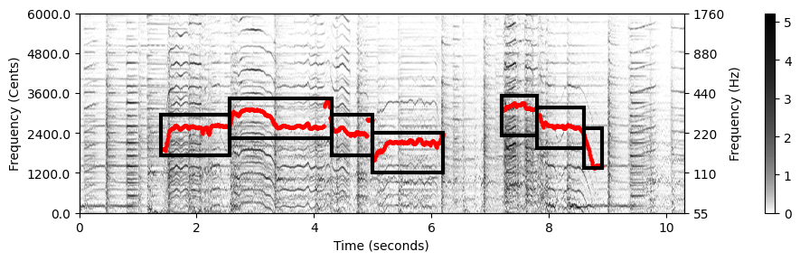
original recordingF0 sonification only멜로디 추출과 분리
멜로디
특정 노래를 설명하라고 하면 메인 멜로디를 부르거나 흥얼거리는 경우가 많다. 일반적으로 멜로디는 특정 음악적 아이디어를 표현하는 음악 톤의 선형적 연속으로 정의될 수 있다. 음색의 특수한 배치로 인해 멜로디는 하나의 일관된 실체로 인식되며, 곡의 가장 기억에 남는 요소로 듣는 이의 머리에 박히게 되며, 멜로디는 일반적으로 어떤 식으로든 두드러진다.
악보에서 멜로디는 높은 음으로 구성되는 경우가 많고 반주는 낮은 음으로 구성되는 경우가 많다. 또는 멜로디가 특징적인 음색을 가진 일부 악기로 연주된다. 일부 연주에서 멜로디의 음은 비브라토, 트레몰로 또는 글리산도(한 음에서 다른 음으로의 연속적인 미끄러짐)와 같이 쉽게 식별할 수 있는 시간-주파수 패턴을 특징으로 한다.
음악 처리의 다른 많은 개념과 마찬가지로 멜로디의 개념은 다소 모호하다.
- 먼저, 음악이 오디오 녹음의 형태로 제공되는 시나리오를 고려한다(상징적 음악 표현이 아님).
- 둘째, 음의 시퀀스를 추정하는 대신 음의 피치에 해당하는 F0-값의 시퀀스로 멜로디를 나타낸다.
- 셋째, 멜로디가 지배적인 음악(예: 리드 싱어 또는 리드 악기 연주)으로 제한한다.
- 넷째, 하나의 음원에 연관될 수 있는 멜로디 라인은 한 번에 하나만 있다고 가정한다.
멜로디 추출 (Melody Extraction)
- 이러한 가정을 바탕으로 멜로디 추출 문제는 다음과 같은 신호 처리 작업으로 간주할 수 있다. 녹음이 주어지면 리드 보이스 또는 악기가 연주하는 음에 해당하는 우세한(predominant) F0 값의 시퀀스를 자동으로 추정하는 것이 목표이다.
- 기본 절차는 다음과 같이 요약할 수 있다.
- 먼저 돌출 표현을 계산한다.
- 그런 다음 적절한 평활화 또는 점수 기반 제약 조건을 사용하여 주요 F0 값의 궤적을 도출한다.
- 또한 Salamo and Gómez가 제안한 것처럼 피치 윤곽에 따라 다른 음악적 제약을 도입할 수도 있다.
- 가정이 단순화된 제약 경우에도 멜로디 추출 문제는 쉽지 않다.
- 많은 악기가 동시에 연주되는 음악에서는 개별 악기의 음에 특정한 시간-주파수 패턴을 부여하기가 어렵다.
- 또한 공명 및 잔향 효과의 존재는 다른 음원의 중첩을 더욱 증가시킨다.
- 또한 기본 주파수를 성공적으로 추정한 후에도 여전히 F0 값 중 어느 것이 주 멜로디에 속하고 반주의 일부인지 결정해야 한다.
- Freischütz 예를 계속하여 다음 그림에 스펙트로그램 표현과 소프라노 가수가 연주하는 멜로디의 F0 궤적을 보여준다.
- 가수가 계속 노래하는 것은 아니다. 이는 스펙트로그램 아래에 표시된 활동 패턴(activity pattern)으로도 알 수 있다.
- 일부 시점에서 가장 높은 크기의 스펙트럼 빈이 반주에 속할 수 있다. 이것이 멜로디 추정 오류의 한 가지 이유이다.
- 일부 고조파는 기본 주파수보다 더 많은 에너지를 포함할 수 있으며, 이로 인해 멜로디 추정에서 옥타브 오류가 발생할 수 있다.
def plot_STFT_F0_activity(Y, traj, figsize=(7,4), ylim = [0, 4000], cmap='gray_r'):
fig, ax = plt.subplots(2, 2, gridspec_kw={'width_ratios': [10, 0.2],
'height_ratios': [10, 1]}, figsize= figsize)
fig_im, ax_im, im = plot_matrix(Y, Fs=Fs/H, Fs_F=N/Fs,
ax=[ax[0,0], ax[0,1]], title='', cmap=cmap);
ax[0,0].set_ylim(ylim)
traj_plot = traj[traj[:, 1] > 0, :]
ax[0,0].plot(traj_plot[:, 0], traj_plot[:, 1], color='r', markersize=4, marker='.', linestyle='');
# F0 activity
activity = np.array(traj[:, 1] > 0).reshape(1, -1)
im = ax[1,0].imshow(activity, aspect='auto', cmap='bwr', clim=[-1, 1])
ax[1,0].set_xticks([])
ax[1,0].set_yticks([])
ax[1,1].axis('off')
plt.tight_layout()
return fig, ax# Load audio
fn_wav = 'FMP_C8_F10_Weber_Freischuetz-06_FreiDi-35-40.wav'
x, Fs = librosa.load(path_data+fn_wav)
#ipd.display(Audio(x, rate=Fs))
# Computation of STFT
N = 2048
H = N//4
X = librosa.stft(x, n_fft=N, hop_length=H, win_length=N, pad_mode='constant')
Y = np.log(1 + np.abs(X))
Fs_feature = Fs/H
T_coef = np.arange(X.shape[1]) / Fs_feature
freq_res = Fs / N
F_coef = np.arange(X.shape[0]) * freq_res
# Load F0 trajectory and and resample to fit to X
fn_traj = 'FMP_C8_F10_Weber_Freischuetz-06_FreiDi-35-40_F0-user-Book.csv'
traj_df = pd.read_csv(path_data+fn_traj, header=0,sep=';',keep_default_na=False)
traj = traj_df.values
Fs_traj = 1/(traj[1,0]-traj[0,0])
traj_X_values = interp1d(traj[:,0], traj[:,1], kind='nearest', fill_value='extrapolate')(T_coef)
traj_X = np.hstack((T_coef[:,None], traj_X_values[:,None]))
# Visualization
figsize=(7,4)
ylim = [0, 4000]
fig, ax = plot_STFT_F0_activity(Y, traj_X, figsize=figsize, ylim=ylim)
plt.show()
# Sonification
soni_mono = sonify_trajectory_with_sinusoid(traj_X, len(x), Fs)
#soni_stereo = np.vstack((x.reshape(1,-1), soni_mono.reshape(1,-1))) # left: x, right: sonification
ipd.display(ipd.Audio(soni_mono, rate=Fs))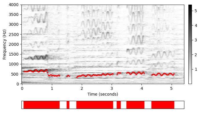
전체 아이디어
단순화된 시나리오에서 멜로디 추출의 목적은 메인 멜로디에 해당하는 F0 값의 시퀀스를 추정하는 것이다. 이와 관련된 작업을 멜로디 분리라고 하며, 음악 신호를 메인 멜로디 음성을 캡처하는 멜로디 구성 요소(melody component)와 나머지 음향 이벤트를 캡처하는 반주 구성 요소(accompaniment component)로 분해하는 것을 목표로 한다.
멜로디 분리의 한 가지 응용은 주어진 노래에 대한 노래방 버전의 자동 생성이다. 여기에서 주요 멜로디 음성은 노래의 원래 녹음에서 제거된다. 좀 더 기술적으로 말하면, 멜로디 분리의 목적은 주어진 신호 \(x\)를 멜로디 성분 \(x^\mathrm{Mel}\)과 반주 성분 \(x^\mathrm{Acc}\)로 분해하는 것이다: \[x = x^\mathrm{Mel} + x^\mathrm{Acc}\]
하나의 일반적인 접근법은 먼저 멜로디 추출 알고리즘을 적용하여 메인 멜로디의 F0-trajectory를 도출하는 것이다. 이러한 F0 값과 해당 고조파를 기반으로 멜로디 구성 요소에 대한 이진 마스크(binary mask)를 구성할 수 있으며 반주의 바이너리 마스크는 보완(complement)으로 정의된다.
HPS에서 설명된 대로 마스킹 기술을 사용하여 두 개의 마스킹된 STFT \(\mathcal{X}^\mathrm{Mel}\) 및 \(\mathcal{X}^\mathrm{Acc}\)를 도출한다. 이로부터 신호 재구성 기법을 적용하여 \(x^\mathrm{Mel}\) 및 \(x^\mathrm{Acc}\) 신호를 얻는다.
이제 이 멜로디 분리 절차를 구현하고 Freischütz 예에 적용해보자.
이진 마스크
- 주어진 F0 궤적에 대해 이진 마스크를 정의하는 방법에는 여러 가지가 있다. 고조파를 고려하여 다음 코드 셀에서 두 가지 변형을 제공한다.
- 첫 번째 변형에서는 허용 오차 매개변수 ‘tol_bin’(주파수 빈으로 주어짐)을 지정할 수 있으며, 이는 각 주파수 빈 주위에 고정 크기의 주파수 이웃을 정의하는 데 사용된다.
- 두 번째 변형에서는 허용 오차 매개변수 ‘tol_cents’(센트 단위로 주어짐)를 지정할 수 있으며, 이는 각 주파수 빈 주위에 주파수 종속 크기의 이웃을 정의하는 데 사용된다. 보다 정확하게는 이웃 크기가 중심 주파수에 따라 선형적으로 증가하며, 따라서 센트 단위로 측정할 때 일정하게 유지된다.
- 다음 그림에서는 두 가지 변형에 대한 멜로디의 이진 마스크(및 반주에 대한 보완)를 보여준다.
def convert_trajectory_to_mask_bin(traj, F_coef, n_harmonics=1, tol_bin=0):
"""Computes binary mask from F0 trajectory
Args:
traj (np.ndarray): F0 trajectory (time in seconds in 1st column, frequency in Hz in 2nd column)
F_coef (np.ndarray): Frequency axis
n_harmonics (int): Number of harmonics (Default value = 1)
tol_bin (int): Tolerance in frequency bins (Default value = 0)
Returns:
mask (np.ndarray): Binary mask
"""
# Compute STFT bin for trajectory
traj_bin = np.argmin(np.abs(F_coef[:, None] - traj[:, 1][None, :]), axis=0)
K = len(F_coef)
N = traj.shape[0]
max_idx_harm = np.max([K, np.max(traj_bin)*n_harmonics])
mask_pad = np.zeros((max_idx_harm.astype(int)+1, N))
for h in range(n_harmonics):
mask_pad[traj_bin*h, np.arange(N)] = 1
mask = mask_pad[1:K+1, :]
if tol_bin > 0:
smooth_len = 2*tol_bin + 1
mask = ndimage.maximum_filter1d(mask, smooth_len, axis=0, mode='constant', cval=0, origin=0)
return mask
def convert_trajectory_to_mask_cent(traj, F_coef, n_harmonics=1, tol_cent=0.0):
"""Computes binary mask from F0 trajectory
Args:
traj (np.ndarray): F0 trajectory (time in seconds in 1st column, frequency in Hz in 2nd column)
F_coef (np.ndarray): Frequency axis
n_harmonics (int): Number of harmonics (Default value = 1)
tol_cent (float): Tolerance in cents (Default value = 0.0)
Returns:
mask (np.ndarray): Binary mask
"""
K = len(F_coef)
N = traj.shape[0]
mask = np.zeros((K, N))
freq_res = F_coef[1] - F_coef[0]
tol_factor = np.power(2, tol_cent/1200)
F_coef_upper = F_coef * tol_factor
F_coef_lower = F_coef / tol_factor
F_coef_upper_bin = (np.ceil(F_coef_upper / freq_res)).astype(int)
F_coef_upper_bin[F_coef_upper_bin > K-1] = K-1
F_coef_lower_bin = (np.floor(F_coef_lower / freq_res)).astype(int)
for n in range(N):
for h in range(n_harmonics):
freq = traj[n, 1] * (1 + h)
freq_bin = np.round(freq / freq_res).astype(int)
if freq_bin < K:
idx_upper = F_coef_upper_bin[freq_bin]
idx_lower = F_coef_lower_bin[freq_bin]
mask[idx_lower:idx_upper+1, n] = 1
return maskfigsize = (12, 2.5)
# Binary masks for melody and accompaniment using bins
tol_bin = 8
mask_mel_bin = convert_trajectory_to_mask_bin(traj_X, F_coef,
n_harmonics=30, tol_bin=tol_bin)
mask_acc_bin = np.ones(mask_mel_bin.shape) - mask_mel_bin
plt.figure(figsize=figsize)
ax = plt.subplot(121)
title = r'Binary mask for melody (tol_bin = %d)'%tol_bin
fig_im, ax_im, im = plot_matrix(mask_mel_bin, Fs=Fs_feature, ax=[ax],
Fs_F=1/freq_res, figsize=figsize, title=title);
plt.ylim(ylim);
ax = plt.subplot(122)
title=r'Binary mask for accompaniment (tol_bin = %d)'%tol_bin
fig, ax, im = plot_matrix(mask_acc_bin, Fs=Fs_feature, ax=[ax],
Fs_F=1/freq_res, figsize=figsize, title=title);
plt.ylim(ylim);
plt.tight_layout()
# Binary masks for melody and accompaniment using cents
tol_cent = 80
mask_mel_cent = convert_trajectory_to_mask_cent(traj_X, F_coef, n_harmonics=30, tol_cent=tol_cent)
mask_acc_cent = np.ones(mask_mel_cent.shape) - mask_mel_cent
plt.figure(figsize=figsize)
ax = plt.subplot(121)
title=r'Binary mask for melody (tol_cent = %d)'%tol_cent
fig_im, ax_im, im = plot_matrix(mask_mel_cent, Fs=Fs_feature, ax=[ax],
Fs_F=1/freq_res, figsize=figsize, title=title);
plt.ylim(ylim);
ax = plt.subplot(122)
title=r'Binary mask for accompaniment (tol_cent = %d)'%tol_cent
fig, ax, im = plot_matrix(mask_acc_cent, Fs=Fs_feature, ax=[ax],
Fs_F=1/freq_res, figsize=figsize, title=title);
plt.ylim(ylim);
plt.tight_layout()
신호 재구성
다음으로 마스크된 STFT \(\mathcal{X}^\mathrm{Mel}\) 및 \(\mathcal{X}^\mathrm{Acc}\) 및 신호 \(x^\mathrm{Mel}\)를 구성한다. 이로부터 신호 재구성 기법을 적용하여 시간 영역 신호 \(x^\mathrm{Acc}\)를 얻는다.
다시 두 가지 마스킹 변형에 대한 결과를 보자.
def compute_plot_display_mel_acc(Fs, X, N, H, mask_mel, figsize=figsize):
mask_acc = np.ones(mask_mel.shape) - mask_mel
X_mel = X * mask_mel
X_acc = X * mask_acc
x_mel = librosa.istft(X_mel, hop_length=H, win_length=N, window='hann', center=True, length=x.size)
x_acc = librosa.istft(X_acc, hop_length=H, win_length=N, window='hann', center=True, length=x.size)
plt.figure(figsize=figsize)
ax = plt.subplot(121)
fig_im, ax_im, im = plot_matrix(np.log(1+10 * np.abs(X_mel)), Fs=Fs_feature, ax=[ax], Fs_F=1/freq_res, figsize=figsize,
title='Masked STFT for melody');
plt.ylim(ylim);
ax = plt.subplot(122)
fig, ax, im = plot_matrix(np.log(1+10 * np.abs(X_acc)), Fs=Fs_feature, ax=[ax], Fs_F=1/freq_res, figsize=figsize,
title='Masked STFT for accompaniment');
plt.ylim(ylim);
plt.show()
audio_player_list([x_mel, x_acc], [Fs, Fs], width=350,
columns=['Reconstructed signal for melody', 'Reconstructed signal for accompaniment'])print('Melody separation (tol_bin = %d)'%tol_bin)
compute_plot_display_mel_acc(Fs, X, N, H, mask_mel_bin, figsize=figsize)
print('Melody separation (tol_cent = %d)'%tol_cent)
compute_plot_display_mel_acc(Fs, X, N, H, mask_mel_cent, figsize=figsize)
mask_mel_joint = np.logical_or(mask_mel_bin, mask_mel_cent)
print('Melody separation (joint mask using "logical or" operator)')
compute_plot_display_mel_acc(Fs, X, N, H, mask_mel_joint, figsize=figsize)Melody separation (tol_bin = 8)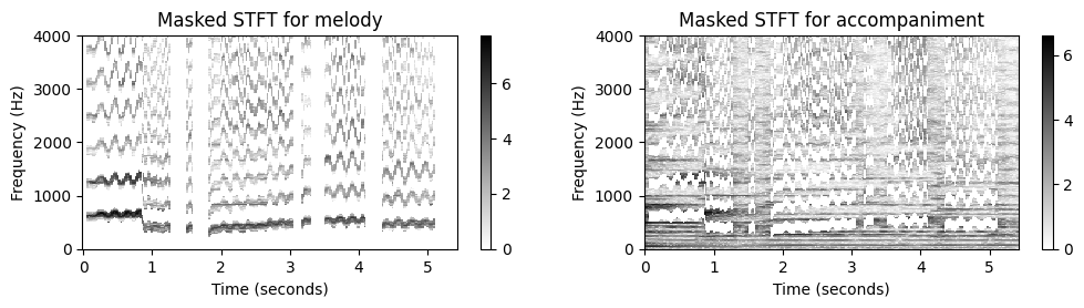
| Reconstructed signal for melody | Reconstructed signal for accompaniment |
|---|---|
Melody separation (tol_cent = 80)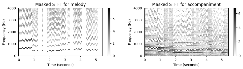
| Reconstructed signal for melody | Reconstructed signal for accompaniment |
|---|---|
Melody separation (joint mask using "logical or" operator)
| Reconstructed signal for melody | Reconstructed signal for accompaniment |
|---|---|
전체과정: 예시
- F0-trajectory가 주어졌다고 가정하면, 멜로디-반주 분리를 위한 전체적인 과정은 다음과 같은 코드 셀로 정리된다. 예로 위에서도 사용했던 Sven Bornemark의 “Stop Messing With Me”에서 발췌 녹음을 보자.
def separate_melody_accompaniment(x, Fs, N, H, traj, n_harmonics=10, tol_cent=50.0):
"""F0-based melody-accompaniement separation
Args:
x (np.ndarray): Audio signal
Fs (scalar): Sampling frequency
N (int): Window size in samples
H (int): Hopsize in samples
traj (np.ndarray): F0 traj (time in seconds in 1st column, frequency in Hz in 2nd column)
n_harmonics (int): Number of harmonics (Default value = 10)
tol_cent (float): Tolerance in cents (Default value = 50.0)
Returns:
x_mel (np.ndarray): Reconstructed audio signal for melody
x_acc (np.ndarray): Reconstructed audio signal for accompaniement
"""
# Compute STFT
X = librosa.stft(x, n_fft=N, hop_length=H, win_length=N, pad_mode='constant')
Fs_feature = Fs / H
T_coef = np.arange(X.shape[1]) / Fs_feature
freq_res = Fs / N
F_coef = np.arange(X.shape[0]) * freq_res
# Adjust trajectory
traj_X_values = interp1d(traj[:, 0], traj[:, 1], kind='nearest', fill_value='extrapolate')(T_coef)
traj_X = np.hstack((T_coef[:, None], traj_X_values[:, None, ]))
# Compute binary masks
mask_mel = convert_trajectory_to_mask_cent(traj_X, F_coef, n_harmonics=n_harmonics, tol_cent=tol_cent)
mask_acc = np.ones(mask_mel.shape) - mask_mel
# Compute masked STFTs
X_mel = X * mask_mel
X_acc = X * mask_acc
# Reconstruct signals
x_mel = librosa.istft(X_mel, hop_length=H, win_length=N, window='hann', center=True, length=x.size)
x_acc = librosa.istft(X_acc, hop_length=H, win_length=N, window='hann', center=True, length=x.size)
return x_mel, x_acc# Load audio
fn_wav = 'FMP_C8_Audio_Bornemark_StopMessingWithMe-Excerpt_SoundCloud_mix.wav'
x, Fs = librosa.load(path_data+fn_wav)
x_duration = len(x)/Fs
fn_wav_track_mel = 'FMP_C8_Audio_Bornemark_StopMessingWithMe-Excerpt_SoundCloud_vocals.wav'
x_track_mel, Fs = librosa.load(path_data+fn_wav_track_mel)
fn_wav_track_acc = 'FMP_C8_Audio_Bornemark_StopMessingWithMe-Excerpt_SoundCloud_accomp.wav'
x_track_acc, Fs = librosa.load(path_data+fn_wav_track_acc)
# Read constraint regions
fn_region = 'FMP_C8_F11_SvenBornemark_StopMessingWithMe_CR.csv'
constraint_region_df = pd.read_csv(path_data+fn_region, header=0, sep=';', keep_default_na=False)
constraint_region = constraint_region_df.values
# Compute trajectory
traj, Z, T_coef, F_coef_hertz, F_coef_cents = compute_traj_from_audio(x, Fs=Fs,
constraint_region=constraint_region, gamma=0.1)
N = 2048
H = N//4
x_mel, x_acc = separate_melody_accompaniment(x, Fs=Fs, N=N, H=H, traj=traj, n_harmonics=30, tol_cent=50)
audio_player_list([x_mel, x_acc], [Fs, Fs], width=350,
columns=['Reconstructed signal for melody', 'Reconstructed signal for accompaniment'])
audio_player_list([x_track_mel, x_track_acc], [Fs, Fs], width=350,
columns=['Ideal signal for melody', 'Ideal signal for melody for accompaniment'])C:\Users\JHCho\AppData\Local\Temp\ipykernel_15196\3605094473.py:23: RuntimeWarning: divide by zero encountered in log2
bin_index = np.floor((1200 / R) * np.log2(F / F_ref) + 0.5).astype(np.int64)| Reconstructed signal for melody | Reconstructed signal for accompaniment |
|---|---|
| Ideal signal for melody | Ideal signal for melody for accompaniment |
|---|---|
결론
음원을 멜로디 성분과 반주 성분으로 분해하는 과정을 제시하였으며, 이때 멜로디의 F0-trajectory가 주어진다고 가정하였다. 분명히 이러한 단순한 음성 분리 시나리오에서는 추출된 F0 값의 정확도에 대한 요구 사항이 매우 높다. 또한, 마찰음 및 파열음 성분(자음에서 유래)과 같은 노래 목소리의 비화성 특성은 고려되지 않았다. 이러한 비고조파 구성 요소를 모델링하고 분리하는 것은 일반적으로 어려운 연구이다.
가창 분리(singing voice separation)에 대한 최근 접근 방식(또는 더 일반적으로 말하면 소스 분리(source separation) 접근 방식)은 대부분 많은 양의 훈련 예제를 사용하는 딥 러닝 기술을 기반으로 한다. 다음은 몇 가지 유용한 링크이다.
출처:
- https://www.audiolabs-erlangen.de/resources/MIR/FMP/C8/C8S2_InstantFreqEstimation.html
- https://www.audiolabs-erlangen.de/resources/MIR/FMP/C8/C8S2_SalienceRepresentation.html
- https://www.audiolabs-erlangen.de/resources/MIR/FMP/C8/C8S2_FundFreqTracking.html
- https://www.audiolabs-erlangen.de/resources/MIR/FMP/C8/C8S2_MelodyExtractSep.html
\(\leftarrow\) 9.1. 화성-타악 분리 (HPS)